Algorithms in Artificial Intelligence: A Necessary Renunciation of the Deterministic Paradigm

Algorithmic Complexity

When analyzing and developing an algorithm, we must take into consideration the issues regarding execution time or time algorithmic complexity. This concept has to do with the number of elementary operations necessary for execution, depending on the size of the input \(n\).

The computational complexity of the algorithm is often specified by the notation Big \(O\). For example, for an algorithm whose execution time depends on the logarithm of the input, we have a computational complexity of \(O(\log(n))\).

From a complexity point of view, not all problems are the same. An important class concerns those solvable in polynomial time (\(P\)). For an algorithm \(\mathcal{A}\) such that \(\mathcal{A}\ \in P\), we have a time complexity of \(O(n^k)\) with \(k>1\).

From the tractability point of view, only problems for which there is a polynomial time resolution algorithm are tractable. Not polynomial ones are intractable and require the development of approximate solution techniques.

Complexity Classes

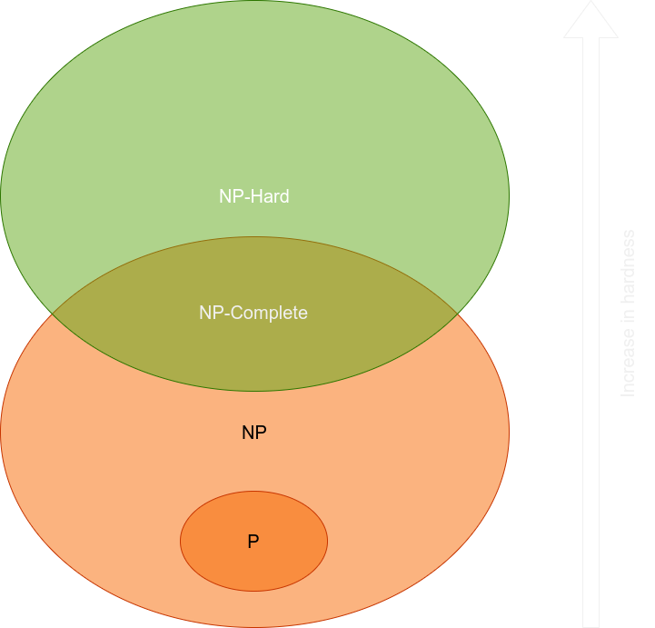
We call \(NP\) problems that allow verification of a given solution in polynomial time on a deterministic Turing machine. An alternative definition is “the set of problems that can be solved in polynomial time by a nondeterministic Turing machine”. It is currently thought that class \(P\) is a subset of class \(NP\). That is, the number of problems solvable in polynomial time is less than the number of problems verifiable in polynomial time. Within the \(NP\) class there is a further complexity class, different from \(P\), called \(NP\)-Complete or \(NPC\), which are the most difficult problems in \(NP\).

\(NPC\) class is intractable (not solvable exactly in polynomial time). We can approach it only approximately. Furthermore, it has the characteristic that if we can solve only one \(NPC\) problem in polynomial time, using the concept of reducibility, we can solve all of them in polynomial time. This is equivalent to the classes \(P\) and \(NP\) being the same. Currently, computer scientists consider this conclusion very unlikely.

The following figure illustrates the relationship between the different complexity classes, according to current knowledge:

An Intractable Example

Verifiability is the key concept. For class \(NP\), given two proposals for acceptable solutions that satisfy the constraints, we can verify in polynomial time which of the two provides the best result.

This last point is of fundamental importance. For class \(NP\) we could think of generating all the possible solutions and using verifiability in polynomial time to keep the best one. However, for problems not solvable in polynomial time, such as many combinatorial ones, we may not be able to generate all possible solutions in a reasonable time.

Let us consider as an example the traveling salesman problem (\(TSP\)), which consists of finding the optimal (minimum) path between \(n\) points (cities) with the constraint of visiting each point only once, starting and ending at the same point. \(TSP\) has the following characteristics:

• \(TSP \in NP\), as each path is verifiable in polynomial time;
• \(TSP \in NPC\), since it is possible to prove that every problem in \(NP\) is reducible to \(TSP\).

Given \(n\) cities, the number of possible circuits is \(\frac{(n-1)!}{2}\). Suppose a sci-fi computer that can calculate a billion routes per second (!). For 50 cities, generating and analyzing all possible circuits would take \(10^{46}\) years. Compare this value with the age of the universe, equal to \(1.5\cdot10^{10}\) years. The analysis of all possible solutions is synonymous with the exact resolution of the problem, so the impossibility of doing this forces us to build approximate procedures.

The Paradigm Shift

An approximate procedure means that a possible algorithm only studies a part of all possible solutions.

At this point, it is worth asking ourselves the following question: how can we know whether we are close to the best possible solution to a problem in the context of an approximate procedure? We cannot, and this is why it is a real change of conceptual paradigm. To estimate the proximity or distance from the global optimum we need, in turn, an approximate algorithm.

Furthermore, if we can only study a part of all the possible solutions, we must restrict the search space. But this restriction must be done with a solid criterion. Otherwise, we risk leaving aside portions of the space of potentially optimal solutions.

Some machine learning algorithms, as evolutionary techniques, are one way of accomplishing this. In practice, they provide a criterion for exploring only some parts of the solution space for the problem. This criterion minimizes the probability that the unexplored portions contain optimal solutions. The only constraint is that the problem belongs to the \(NP\) class. That is, given a proposed solution, we can verify it in polynomial time.