Buddha Elemental 3D - https://unsplash.com/photos/a-black-background-with-green-lines-and-a-black-background-ssYCZwx9CzA
Table of Contents
Introduction
Hopfield networks are a type of artificial neural network designed to mimic the brain’s ability to store and recall patterns, acting like an associative memory system. They consist of fully interconnected neurons that settle into stable states representing stored memories, even when starting from incomplete or noisy inputs.
Core Concept
Introduced by physicist John Hopfield in 1982, these networks treat neurons as simple units that each hold a binary state, such as on or off, with symmetric connections between them that strengthen or weaken signals like synapses in the brain. The key innovation is their collective behavior: instead of processing information sequentially, the entire network evolves together until it reaches one of a few stable configurations, which serve as the stored patterns or memories. This allows the network to complete partial patterns, correct distortions, or retrieve full memories from fragments, much like human recall.
Path to the Energy Idea
Hopfield, trained in physics, drew inspiration from statistical mechanics, particularly the study of spin glasses—disordered magnetic systems where atomic spins align into stable but complex patterns. He saw parallels to neural memory: just as spins in these materials settle into low-energy configurations after interactions, neurons could too. Building on earlier work like the Sherrington-Kirkpatrick spin glass model from 1975, Hopfield adapted it to neural networks by ensuring symmetric connections, which naturally guide the system downhill.
Energy Concept
Hopfield introduced energy as a single global measure of the network’s state, picturing it like a landscape of hills and valleys where each configuration has a height representing its energy level. The network’s update rule—neurons flipping states based on inputs from others—always moves it toward lower energy, guaranteeing convergence to a stable valley, or memory state, without cycles or chaos in most cases. He arrived at this by recognizing that physical systems minimize energy spontaneously, so embedding this principle ensured reliable memory storage and retrieval emerged from simple local rules. Memories become the deepest valleys, attracting nearby states for robust recall.
The Discrete Case
Hopfield’s Theorem demonstrates the convergence of networks that bear his name. If a Hopfield network is perturbed, it passes through a series of states until it reaches a new equilibrium state, corresponding to a minimum energy. The discrete version dates back to 1982.
Consider a Hopfield network made up of neurons that can produce outputs of +1 or -1, with symmetric weights without each neuron feeding itself back (connections come exclusively from other neurons). For n neurons, the weight matrix is
\left(\begin{array}{cccc}
0 & w_{12} & \cdots & w_{1n}\\
w_{21} & 0 & \cdots & w_{2n}\\
\vdots & \vdots & \vdots & \vdots\\
w_{n1} & w_{n2} & \cdots & 0
\end{array}\right).
We assume that the weight updating is given by Hebb’s rule
w_{ij}=y_{i}y_{j},where y_i is the output of the i-th neuron. The weight matrix is given by
\mathbf{W}=\mathbf{y}^{\intercal}\mathbf{y}-\mathbf{I=}\left(\begin{array}{cccc}
0 & y_{1}y_{2} & \cdots & y_{1}y_{n}\\
y_{2}y_{1} & 0 & \cdots & y_{2}y_{n}\\
\vdots & \vdots & \vdots & \vdots\\
y_{n}y_{1} & y_{n}y_{2} & \cdots & 0
\end{array}\right),
where the unitary matrix \mathbf{I} is used to turn off the self-connections and obtain a weight matrix with all the elements of the main diagonal set to zero.
The update of neuron i, i.e., the output at time \tau+1, depends on the outputs at time \tau of all the neurons to which it is connected and on their weights. Hopfield’s update rule dictates
\begin{equation}y^{(\tau+1)}_{i}=\left\{ \begin{array}{ll}
y^{(\tau)}_{i} & \text{{for}\,}y^{(\tau)}_{i}h_{i}>0\\
-y^{(\tau)}_{i} & \text{{for}\,}y^{(\tau)}_{i}h_{i}<0
\end{array}\right.,\end{equation}
where h_i is called the field of the neuron i and corresponds to the sum
h_i=\sum_{j\neq i}w_{ij}y_{j}.From equation (1) we can conclude that the updating of neuron i depends exclusively on the sign of the field
\begin{equation}y^{(\tau+1)}_{i}=\operatorname{sgn}\left(h_{i}\right).\end{equation}Hopfield defines energy as
E=-\frac{1}{2}\sum_{i}\sum_{j\neq i}w_{ij}y_{i}y_{j}.In the case of symmetric weight matrices, the energy reduces to
\begin{equation}E=-\sum_{i}\sum_{j\ > i}w_{ij}y_{i}y_{j}.\end{equation}This energy is a simplified, unbiased version, of the energy actually proposed by Hopfield, given by
E=-\frac{1}{2}\sum_{i}\sum_{j}w_{ij}y_{i}y_{j}-\sum_{i}\theta_{i}y_{i},where \theta_i is the bias of the i-th neuron. This equation is formally identical to the Hamiltonian of the Ising model, developed in the field of statistical physics
E=-\sum_{i}\sum_{j}J_{ij}\sigma_{i}\sigma_{j}-\sum_{i}h_{i}\sigma_{i},with the following correspondences in the symbols
| Ising | Hopfield |
| Spin \sigma_i | Neuron y_i |
| Coupling J_{ij} | Weights w_{ij} |
| Field h_i | Bias \theta_i |
| Magnetic energy | Network energy |
What Hopfield was looking for was a neural network that could be analyzed mathematically, consistently converged, and could memorize patterns and recover them from noisy inputs. Hopfield’s profound insight was the realization that the Ising model possessed these properties and could therefore model a neural network through a physical analogy, which led him directly to the concept of network energy.
Let’s consider this last case and see how the energy varies with the variation in the output of a neuron k. We can separate the expression (3) into two parts, one relating to the neuron k and one relating to all the others.
E=-y_{k}\sum_{j\neq k}w_{kj}y_{j}-\sum_{i\neq k}\sum_{j>i}w_{ij}y_{i}y_{j}.We can obtain two energies relating to the situations before and after the interaction of the neuron k with all the other neurons
E^{(\tau)}=-y^{(\tau)}_{k}\sum_{j\neq k}w_{kj}y_{j}-\sum_{i\neq k}\sum_{j>i}w_{ij}y_{i}y_{j}E^{(\tau+1)}=-y^{(\tau+1)}_{k}\sum_{j\neq k}w_{kj}y_{j}-\sum_{i\neq k}\sum_{j>i}w_{ij}y_{i}y_{j},and the energy change is
\begin{equation}\Delta E=-\left(y^{(\tau+1)}_{k}-y^{(\tau)}_{k}\right)\sum_{j\neq k}w_{kj}y_{j}=-\left(y^{(\tau+1)}_{k}-y^{(\tau)}_{k}\right)h_i.\end{equation}We have two cases, given by whether the outputs of y_k^{\tau+1} and y_k^{\tau} are equal or different. If they are equal, the energy variation is zero. If they are different, using equation (2), we have that
\operatorname{sgn}\left(y^{(\tau+1)}_{i}\right)=-\operatorname{sgn}\left(y^{(\tau)}_{i}\right)=\operatorname{sgn}\left(h_{i}\right).Applying this relation to equation (4) we get
\boxed{\operatorname{sgn}\left(\Delta E\right)=-\left[\operatorname{sgn}\left(h_{i}\right)-\left(-\operatorname{sgn}\left(h_{i}\right)\right)\right]\left[\operatorname{sgn}\left(h_{i}\right)\right]=-2\left[\operatorname{sgn}\left(h_{i}\right)\right]^{2}}.Therefore, in the case of a change in state of the neuron k, the energy change is negative, meaning it always decreases. Since in the case of no change in state results \Delta E=0, the energy in a Hopfield network can never increase. This conclusion implies that the network will necessarily reach a stable state in which the energy cannot be further reduced, given that the number of possible states is finite.
When the network experiences a perturbation, an energy minimization process is then initiated until the network reaches the stable state.
The Continuous Case
The proof in the continuous case is more complex but reaches the same conclusion. Hopfield considers his network as a dynamic system and tries to understand whether it will stabilize or not.
Lyapunov Functions
Suppose we have a dynamical system defined as
\frac{dx}{dt}=f(x),where x(t) is the state of the system. A function V(x) is called a Lyapunov function if:
- V(x)\geq0 for any x;
- V(x)=0 only at the equilibrium x=x^*;
- The derivative along the trajectories is non-positive:
\frac{dV}{d\tau}=\nabla V\cdotp\frac{dx}{d\tau}=\nabla V\cdotp f(x)\leq0.Lyapunov functions are primarily used to study the stability of dynamical systems without having to explicitly solve the equations of motion.
Simply put, they help us understand whether a system tends to remain close to a state of equilibrium or whether it moves away from it.
Network Dynamics
To obtain the dynamics of the network, we can use a physical analogy with RC circuits. For a capacitor C_i with resistance R_i, Kirchhoff’s law is
C_{i}\frac{du_{i}}{d\tau}=-\frac{u_{i}}{R_{i}}+\sum_{j}w_{ij}y_{j}+I_{i},where
- u_i is the capacitor voltage;
- C_i is the capacitance of the capacitor, equal to the ratio between the charge q_i and u_i;
- \sum_{j}w_{ij}y_{j}+I_{i} is the input current.
In this system the capacitor accumulates charge at rate C_{i}\frac{du_{i}}{d\tau} while the resistor causes a discharge given by -\frac{u_{i}}{R_{i}}.
This same dynamic allows a biological interpretation if we consider
- u_i is the membrane potential;
- y_i=g(u_i) is the firing rate (output);
- \sum_{j}w_{ij}y_{j}+I_{i} is the input from connected neurons;
- \frac{-u_{i}}{R_{i}} is the natural tendency of the neuron to return to the resting potential.
Kirchhoff’s dynamics, in its biological version, is a simplification of the Hodgkin-Huxley model, which is essentially an application of Kirchhoff’s laws to neuronal membranes with dynamic ionic conductances. This work, carried out in 1952, earned them the Nobel Prize in Physiology or Medicine in 1963.
Proof of the Theorem
The Hodgkin-Huxley model derives directly from Kirchhoff but produces non-gradient dynamics (there is no simple Lyapunov function, and it can give rise to limit cycles). Hopfield simplifies the framework to obtain dissipative dynamics with an explicit Lyapunov function. Therefore, he does not start from a biophysically faithful model but from a simplified one given by some strong conditions, such as symmetric weights, monotone neurons, and linear RC dynamics. In this way, he simplifies the mathematical treatment and obtains a configuration in which convergence is guaranteed.
The continuous version is later than the discrete one, dating back to 1984. Here too, Hopfield puts a brilliant idea into practice, combining the Ising model with the dynamics of RC circuits given by Kirchhoff’s law. The Ising model provides the concepts of the system’s global energy, minima (stable states), and attractors interpreted as memory states; the circuit dynamics allows for a continuous model with a Lyapunov function at its core. The result is a neural network that relaxes toward energy minima like a magnetic system.
So, this whole discussion allows us to justify the dynamics used by Hopfield, a “Kirchhoff-style” dynamic
\begin{equation}\frac{du_{i}}{d\tau}=-u_{i}+\sum_{j}w_{ij}y_{j}+I_{i},\end{equation}where we consider C_{i}=R_i=1 to simplify the mathematical formalism. u_i is the net input of the neuron, linked to the output of the actual neuron through a monotonic function: the activation function
\begin{equation}y_i =g(u_i);u_i=g^{-1}(y_i).\end{equation}For Hopfiled, the Lyapunov function is the energy of the network, defined as
E=-\frac{1}{2}\sum_{i}\sum_{j}w_{ij}y_{i}y_{j}+\sum_{i}\int^{y_{i}}_{0}g^{-1}(s)\,ds-\sum_{i}I_{i}y_{i}.Using the chain rule, the time variation of energy can be expressed as
\frac{dE}{d\tau}=\sum_{i}\frac{\partial E}{\partial y_{i}}\frac{dy_{i}}{d\tau}.Taking advantage of the symmetry of the weight matrix \mathbf{W}, we have
\begin{equation}\frac{\partial E}{\partial y_{i}}=u_{i}-\left(\sum_{j}w_{ij}y_{j}+I_{i}\right).\end{equation}Considering equation (6), this expression stems from the relation
\frac{d}{dy_{i}}\left(\int^{y_{i}}_{o}g^{-1}_{i}(s)\,ds\right)=g^{-1}(y_{i})=u_{i}.The term in parentheses in the right-hand side of equation (7) can be derived from the dynamics of the network (5), by making a small rearrangement of the terms
\sum_{j}w_{ij}y_{j}+I_{i},=\frac{du_{i}}{d\tau}+u_{i},resulting
\frac{\partial E}{\partial y_{i}}=-\frac{du_{i}}{d\tau}.Given that, from equation (6)
\frac{dy_{i}}{d\tau}=g'(u_{i})\frac{du_{i}}{d\tau},the derivative of energy becomes
\boxed{\frac{dE}{d\tau}=-\sum_{i}\left(\frac{du_{i}}{d\tau}\right)\frac{dy_{i}}{d\tau}=-\sum_{i}g'(u_{i})\left(\frac{du_{i}}{d\tau}\right)^{2}\leq 0}.The energy variation is never positive, since we considered g(u_i) monotone, so its derivative is positive.
It is important to emphasize that this derivation requires symmetric weight matrices, the only ones that guarantee that the energy is a Lyapunov function, thus ensuring convergence.
Memory and Data Reconstruction
A Hopfield network can be thought of as a landscape filled with hills and valleys. Each valley represents a memory that the network has stored, such as an image, a word, or any pattern of activity across its neurons. The hills and ridges correspond to unstable or spurious states that the network wants to avoid. When you give the network an input, it is as if you are placing a ball somewhere on this landscape. The ball may start in a random spot, but the shape of the landscape naturally guides it down into the nearest valley. That valley corresponds to the memory closest to the input you provided.
The network creates these valleys when it stores patterns. Each pattern shapes the landscape so that its corresponding valley is deep and stable. The deeper the valley, the more reliably the network can reach that memory from nearby starting points. This is why a Hopfield network can recover incomplete or corrupted data. For example, if the network has memorized the word “CAT” and you provide an input like “C_T” or a version with some errors, the neurons collectively adjust their states, as if the ball were rolling downhill. The network gradually settles into the valley corresponding to the original pattern, effectively reconstructing the complete memory.
However, the network is not perfect. If too many patterns are stored, the landscape can develop extra, unintended valleys, which are called spurious states. These are local minima that do not correspond to any memory you intended to store, and the network might sometimes settle there instead. This limitation defines the network’s capacity: for a network of binary neurons, it can reliably store roughly 13–14% of its total number of neurons in patterns.
The key idea is that memory in a Hopfield network is not like a simple list of items. Instead, memories exist as attractors in a dynamic system. Corrupted or incomplete inputs are just starting points in the landscape, and the network’s dynamics naturally guide the system toward the attractor that represents the stored pattern. The neurons update their states collectively, not in isolation, and this global coordination is what allows the network to reconstruct memories accurately. In other words, a Hopfield network remembers like a ball finding its way to the deepest valley: even if it starts in the wrong place, the shape of the landscape ensures it ends up in the correct position, restoring the memory.
Conclusion
John Hopfield did receive the Nobel Prize in Physics in 2024, and he shared it with Geoffrey Hinton. They were awarded this prize on October 8 2024.
The Nobel Committee recognized them “for foundational discoveries and inventions that enable machine learning with artificial neural networks,” highlighting how their work from the 1980s laid the groundwork for today’s powerful AI technologies.
Hopfield was specifically cited for developing the associative memory model (now called Hopfield networks) that can store and reconstruct patterns, drawing on ideas from physics—in particular the energy landscapes used in models like Ising—and applying them to information processing.
Hinton was recognized for subsequent advances, especially through models like the Boltzmann machine, that enabled neural networks to learn complex data representations. Together, their contributions helped transform neural networks from theoretical constructs into the foundation of modern machine learning.
The work of these researchers represents a milestone showing how deeply ideas about memory and learning in networks have influenced science and technology.
Hopfield’s results constitute a milestone in the development of neural network theory. It is important, beyond the theory itself, because it provides an example of how physical concepts can guide theory in the development of new machine learning methods. Personally, I am convinced that if one day we can achieve Artificial General Intelligence (AGI), it will be possible by introducing methods and insights that are not strictly statistical but physical. As Hopfield and Hinton did.