Entropy: A Comprehensive Guide From Information Theory to Machine Learning

Introduction: The Genesis of Information Theory

The mathematical foundation of modern digital communication, data science, and theoretical computer science was established in 1948 with Claude E. Shannon’s seminal paper, A Mathematical Theory of Communication, published in the Bell System Technical Journal. Working as a mathematician and cryptographer at Bell Telephone Laboratories, Shannon addressed a primary engineering challenge: how to reliably quantify, encode, transmit, and compress information over noisy physical channels, independent of the semantic context or subjective meaning of the underlying message. As Shannon famously stated at the beginning of his work,

“The semantic aspects of communication are irrelevant to the technical problem.”

— Claude Shannon

What mattered fundamentally was not what was being said, but the statistical properties of the choices available within a defined message space.

Historically, the structural formulation of information quantification owes a substantial theoretical debt to 19th-century statistical mechanics. When Shannon was formalizing a measure for the uncertainty or “lack of predictability” inherent in a discrete probability distribution, he arrived at a logarithmic function of probabilities. According to historical accounts, Shannon hesitated on how to name this critical quantity. It was the mathematician and physicist John von Neumann who suggested calling it entropy. Von Neumann observed that Shannon’s probabilistic expression possessed the exact mathematical structural identity as Ludwig Boltzmann’s H-theorem in physical thermodynamics, famously adding,

“You should call it entropy, for two reasons. In the first place, your uncertainty function has been used in statistical mechanics under that name, so it already has a name. In the second place, and more important, no one really knows what entropy is, so in a debate you will always have the advantage.”

— John von Neumann

While classical thermodynamic entropy measures missing physical information regarding the microscopic state (positions and momenta of particles) of a macroscopically observed physical system, information-theoretic entropy measures the inherent unpredictability, surprise, and absolute information volume associated with random variables and stochastic processes.

In contemporary computer science, entropy transcends telecommunication networks and bit-rate constraints. It serves as the primary metric in several key domains:

• Data Compression & Algorithm Analysis: It sets the theoretical lower bound on lossless data compression, as proved by Shannon’s Source Coding Theorem, dictating the maximal efficiency achievable by algorithms like Huffman coding, LZ77, and arithmetic coding.
• Machine Learning & Artificial Intelligence: It provides the foundation for decision tree induction criteria (via Information Gain), governs the optimization of probabilistic classifiers through cross-entropy loss functions, and defines bounds on generative model alignment using Kullback-Leibler (KL) divergence.
• Theoretical Computer Science & Complexity: It dictates bounds on search algorithms, dictionary data structures, and randomized algorithms, where the entropy of the search space places a hard lower limit on the decision-tree height required to identify specific elements.
• Physics & Quantum Information: It establishes fundamental limits in physical measurement, non-equilibrium statistical mechanics, and quantum computing through entropic formulations of the Heisenberg Uncertainty Principle and von Neumann quantum entropy.

To build a rigorous understanding of entropy, one must trace its development chronologically and mathematically: starting from combinatorial counting over discrete symbol spaces, expanding through the analytical properties of continuous probability density functions, exploring multi-variable relationships, and investigating modern applications in computational theory and deep learning.

Combinatorial Entropy: From Permutations to Binary Encoding

To establish a completely rigorous foundation for information entropy without presupposing probabilistic measure spaces, we must begin with combinatorial principles over discrete message spaces.

Information, at its core, is tied to the concept of selection from a set of possible microstates or symbol arrangements. By analyzing how the number of valid permutations scales with sequence length and symbol composition, we can naturally derive a measure for information capacity per symbol.

Consider a discrete alphabet \Sigma = { \sigma_1, \sigma_2, \dots, \sigma_L } containing L distinct symbols. Suppose we assemble a sequence of total length N constructed exclusively from elements of \Sigma. Within this sequence, let n_i denote the multiplicity (the absolute frequency of occurrence) of the symbol \sigma_i for each i \in {1, 2, \dots, L}. Because the sequence consists of exactly N total elements, the sum of all individual symbol multiplicities must equal N:

\sum_{i=1}^{L} n_i = N

If all symbols in the sequence were unique, the total number of distinct arrangements (permutations) would simply be N!. However, since all instances of a given symbol \sigma_i are structurally indistinguishable from one another, permuting two identical symbols does not yield a novel sequence. To account for this overcounting, we divide N! by the product of the factorial multiplicities of each distinct symbol type. The total number of unique, distinguishable permutations P that can be constructed is precisely defined by the multinomial coefficient:

P(N; n_1, n_2, \dots, n_L) = \frac{N!}{n_1! n_2! \dots n_L!} = \frac{N!}{\prod_{i=1}^{L} n_i!}

The quantity P represents the cardinality of the configuration space—that is, the total number of distinct messages that share the same symbol composition vector \mathbf{n} = (n_1, n_2, \dots, n_L).

Now, consider the problem from a fundamental computer science perspective: how many bits of binary storage are required to uniquely identify and encode each of these P distinct permutations?
Suppose we employ a fixed-length binary encoding scheme using a string of length b bits. A binary code of length b has a total capacity of 2^b distinct state representations (since each bit position independently offers 2 choices, yielding 2 \times 2 \times \dots \times 2 = 2^b combinations). To guarantee that every single permutation among the P possibilities maps to a unique binary code without ambiguity or collision, the encoding capacity must at least match the number of permutations:

2^b = P

To isolate the required number of bits b, we apply the base-2 logarithm to both sides of the equation:

\log_2(2^b) = \log_2 P

b = \log_2 P

Substituting the multinomial coefficient for P into this logarithmic expression yields the total binary representation length required for the entire sequence of N symbols:

b = \log_2 \left( \frac{N!}{\prod_{i=1}^{L} n_i!} \right)

Using standard logarithmic identities—specifically the quotient rule \log_2(A/B) = \log_2 A - \log_2 B and the product rule \log_2(\prod_i A_i) = \sum_i \log_2 A_i—we can decompose this total bit count into an explicit difference of logarithmic factorials:

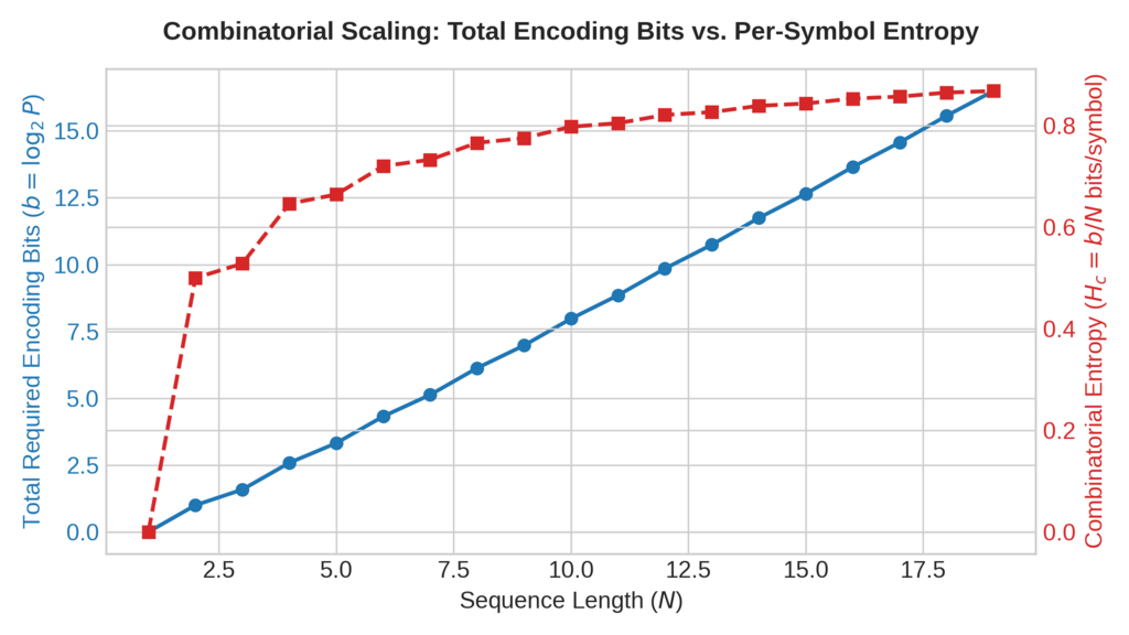
b = \log_2(N!) - \log_2 \left( \prod_{i=1}^{L} n_i! \right)

b = \log_2(N!) - \sum_{i=1}^{L} \log_2(n_i!)

While b represents the total information content of the entire sequence of length N in bits, it is far more informative to determine the average information density per individual symbol. We define combinatorial entropy, denoted as H_c, as the ratio of the total required encoding bit length b to the sequence length N:

H_c = \frac{b}{N} = \frac{1}{N} \log_2 P

H_c = \frac{1}{N} \left[ \log_2(N!) - \sum_{i=1}^{L} \log_2(n_i!) \right]

The units of H_c are strictly expressed in bits per symbol.

Physical and operational interpretation of H_c:

• Encoding Efficiency Boundary: H_c represents the minimum average number of bits per symbol that any fixed-length permutation-based encoding algorithm must allocate to uniquely represent sequences with symbol composition vector \mathbf{n}.
• Combinatorial State Density: When all symbols are identical (n_1 = N, n_{i \neq 1} = 0), P = 1 and H_c = \frac{\log_2 1}{N} = 0 bits/symbol, reflecting zero uncertainty and zero information choice. Conversely, when symbols are evenly distributed, P reaches its combinatorial maximum, maximizing H_c.

Deriving Shannon Entropy via Stirling’s Approximation

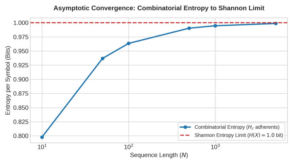
While combinatorial entropy H_c provides a concrete, permutation-based counting framework for measuring information content, evaluating factorial expressions like N! for massive data sequences becomes computationally intractable. To bridge combinatorial enumeration and probabilistic modeling, Claude Shannon utilized Stirling’s approximation, which provides an asymptotic expansion for the logarithm of factorials when N is sufficiently large.

The Asymptotic Expansion of Factorials

Stirling’s formula approximates the factorial of a large integer N through the expression:

N! \approx \sqrt{2\pi N} \left(\frac{N}{e}\right)^N

Taking the natural logarithm of both sides yields the standard logarithmic form used in information theory:

\ln(N!) \approx N \ln N - N + \frac{1}{2} \ln(2\pi N)

For huge sequence lengths (N \to \infty), the dominant terms govern the growth rate, allowing us to drop lower-order corrections and write the primary approximation:

\ln(N!) \approx N \ln N - N

Step-by-Step Derivation of Shannon Entropy

Let us return to our natural-logarithm version of combinatorial entropy, denoted as H_c^{\ln}, which measures information density in natural units (nats per symbol):

H_c^{\ln} = \frac{1}{N} \ln P = \frac{1}{N} \left[ \ln(N!) - \sum_{i=1}^{L} \ln(n_i!) \right]

Applying Stirling’s approximation \ln(x!) \approx x \ln x - x to both the total sequence factorial \ln(N!) and each individual symbol multiplicity factorial \ln(n_i!):

\ln(N!) \approx N \ln N - N

\ln(n_i!) \approx n_i \ln n_i - n_i

Substituting these approximations back into the combinatorial entropy equation gives:

H_c^{\ln} \approx \frac{1}{N} \left[ (N \ln N - N) - \sum_{i=1}^{L} (n_i \ln n_i - n_i) \right]

Expanding the summation and distributing terms:

H_c^{\ln} \approx \frac{1}{N} \left[ N \ln N - N - \sum_{i=1}^{L} n_i \ln n_i + \sum_{i=1}^{L} n_i \right]

Because the total sequence length N is defined as the sum of all individual symbol frequencies (\sum_{i=1}^{L} n_i = N), the positive linear sum \sum_{i=1}^{L} n_i directly cancels out with the negative term -N:

H_c^{\ln} \approx \frac{1}{N} \left[ N \ln N - \sum_{i=1}^{L} n_i \ln n_i \right]

Dividing through by N:

H_c^{\ln} \approx \frac{N \ln N}{N} - \sum_{i=1}^{L} \frac{n_i}{N} \ln n_i = \ln N - \sum_{i=1}^{L} \frac{n_i}{N} \ln n_i

We can rewrite the leading term \ln N by multiplying it by \sum_{i=1}^{L} \frac{n_i}{N}, which evaluates identically to 1 since the probabilities sum to unity:

\ln N = \ln N \cdot \left( \sum_{i=1}^{L} \frac{n_i}{N} \right) = \sum_{i=1}^{L} \frac{n_i}{N} \ln N

Substituting this back into our expression and combining terms under a single unified summation:

H_c^{\ln} \approx \sum_{i=1}^{L} \frac{n_i}{N} \ln N - \sum_{i=1}^{L} \frac{n_i}{N} \ln n_i

H_c^{\ln} \approx \sum_{i=1}^{L} \frac{n_i}{N} \left( \ln N - \ln n_i \right) = -\sum_{i=1}^{L} \frac{n_i}{N} \left( \ln n_i - \ln N \right) = -\sum_{i=1}^{L} \frac{n_i}{N} \ln \left( \frac{n_i}{N} \right)

Recognizing that the ratio \frac{n_i}{N} represents the empirical relative frequency—or probability p_i—of the i-th symbol occurring within sequence length N, we substitute p_i = \frac{n_i}{N} to establish the general continuous asymptotic limit:

H(X) = -\sum_{i=1}^{L} p_i \ln p_i

Converting from natural logarithms (nats) to base-2 logarithms (bits) via the standard change-of-base rule (\log_2 x = \frac{\ln x}{\ln 2}), we arrive at the classic formulation of Shannon Entropy:

H(X) = -\sum_{i=1}^{L} p_i \log_2 p_i

Asymptotic Bound and Properties

Due to the approximations introduced by dropping Stirling’s lower-order terms, information entropy acts as an upper bound to combinatorial entropy (H \ge H_c). Shannon entropy completely abstracts away sequence ordering, structural positioning, and absolute dataset scale, depending strictly and exclusively on the underlying probability distribution P(X).

Differential Entropy and Continuous Probability Densities

When moving from discrete symbol distributions to continuous random variables, Claude Shannon extended discrete entropy by replacing finite summations over discrete probabilities with definite integrals over probability density functions (PDFs). This continuous metric is termed differential entropy (or continuous entropy) and is denoted by h(X).

Formal Definition of Differential Entropy

Let X be a continuous random variable defined over a continuous support domain \mathcal{X} \subseteq \mathbb{R}, governed by a probability density function p(x) satisfying the normalization axiom \int_{\mathcal{X}} p(x) , dx = 1. The differential entropy h(X), measured in nats (when using natural logarithms) or bits (when using base-2 logarithms), is defined as:

h(X) = -\int_{-\infty}^{\infty} p(x) \ln p(x) \, dx = \mathbb{E}_{X}[-\ln p(X)]

In base-2 units, the corresponding formulation becomes:

h(X) = -\int_{-\infty}^{\infty} p(x) \log_2 p(x) \, dx

While differential entropy retains a structural resemblance to discrete Shannon entropy, replacing discrete probabilities p_i \in [0, 1] with density values p(x) \in [0, \infty) introduces fundamental mathematical differences that require careful analysis.

Complete Analytical Derivation of Gaussian Differential Entropy

To understand the continuous properties of differential entropy, consider one of the most important continuous distributions in probability theory: the univariate Gaussian (Normal) distribution \mathcal{N}(\mu, \sigma^2).

The PDF of a continuous Gaussian random variable X with mean \mu and variance \sigma^2 is given by:

p(x) = \frac{1}{\sqrt{2\pi\sigma^2}} \exp\left( -\frac{(x-\mu)^2}{2\sigma^2} \right)

To derive its differential entropy h_{\mathcal{N}}(X), we substitute this density function directly into the continuous entropy integral:

h_{\mathcal{N}}(X) = -\int_{-\infty}^{\infty} p(x) \ln \left[ \frac{1}{\sqrt{2\pi\sigma^2}} \exp\left( -\frac{(x-\mu)^2}{2\sigma^2} \right) \right] dx

Applying logarithmic product and power identities ($\ln(A \cdot B) = \ln A + \ln B$ and $\ln(e^k) = k$), we expand the logarithmic term inside the integrand:

\ln p(x) = \ln \left( (2\pi\sigma^2)^{-1/2} \right) + \ln \left( \exp\left( -\frac{(x-\mu)^2}{2\sigma^2} \right) \right)

\ln p(x) = -\frac{1}{2} \ln(2\pi\sigma^2) - \frac{(x-\mu)^2}{2\sigma^2}

Substituting this expression back into the differential entropy integral:

h_{\mathcal{N}}(X) = -\int_{-\infty}^{\infty} p(x) \left[ -\frac{1}{2} \ln(2\pi\sigma^2) - \frac{(x-\mu)^2}{2\sigma^2} \right] dx

Distributing the integrand yields two distinct integral terms:

h_{\mathcal{N}}(X) = \frac{1}{2} \ln(2\pi\sigma^2) \int_{-\infty}^{\infty} p(x) \, dx + \frac{1}{2\sigma^2} \int_{-\infty}^{\infty} (x-\mu)^2 p(x) \, dx

We can evaluate both integrals using standard probabilistic definitions:

• The first integral \int_{-\infty}^{\infty} p(x) , dx integrates the PDF over its entire domain, which equals 1 by the total probability axiom.
• The second integral \int_{-\infty}^{\infty} (x-\mu)^2 p(x) , dx matches the formal definition of variance \mathbb{E}[(X-\mu)^2] = \sigma^2.

Substituting these structural values back into the equation:

h_{\mathcal{N}}(X) = \frac{1}{2} \ln(2\pi\sigma^2) \cdot (1) + \frac{1}{2\sigma^2} \cdot (\sigma^2)

Using the identity \frac{1}{2} = \ln(e^{1/2}) = \frac{1}{2}\ln(e), we can combine both logarithmic terms:

h_{\mathcal{N}}(X) = \frac{1}{2} \ln(2\pi\sigma^2) + \frac{1}{2} \ln(e) = \frac{1}{2} \ln(2\pi e \sigma^2)

Converting to base-2 logarithms (bits) via the change-of-base formula ($\log_2 x = \frac{\ln x}{\ln 2}$), we arrive at the final analytical expression for Gaussian differential entropy:

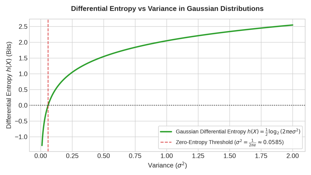
h_{\mathcal{N}}(X) = \frac{1}{2} \log_2 (2\pi e \sigma^2)

Theoretical Anomalies: Negative Entropy and Non-Invariance under Scale

Negative Differential Entropy

Examining the derived Gaussian entropy equation h_{\mathcal{N}}(X) = \frac{1}{2} \ln(2\pi e \sigma^2), we observe that if the variance \sigma^2 is constrained such that:

2\pi e \sigma^2 < 1 \implies \sigma^2 < \frac{1}{2\pi e} \approx 0.0585

the logarithm yields a negative value, resulting in negative differential entropy (h(X) < 0).

This occurs because probability density functions p(x) can exceed 1 over small regions (provided the overall integral remains 1). When p(x) > 1, the logarithmic term \ln p(x) becomes positive, turning -\int p(x) \ln p(x) dx negative. Consequently, differential entropy does not measure absolute information volume, but rather density relative to a uniform reference measure over the real line.

Lack of Invariance under Variable Transformation

Discrete entropy is invariant under bijective coordinate transformations—relabeling discrete symbols does not alter uncertainty. In contrast, differential entropy changes under linear scaling.

Consider scaling a continuous random variable X by a constant non-zero scalar a, defining Y = aX. The PDF of Y is p_Y(y) = \frac{1}{|a|} p_X\left(\frac{y}{a}\right). Evaluating the differential entropy of Y:

h(Y) = -\int_{-\infty}^{\infty} p_Y(y) \ln p_Y(y) \, dy = -\int_{-\infty}^{\infty} \frac{1}{\vert{}a\vert{}} p_X\left(\frac{y}{a}\right) \ln \left( \frac{1}{\vert{}a\vert{}} p_X\left(\frac{y}{a}\right) \right) dy

Using the substitution x = \frac{y}{a} (hence dy = |a| dx):

h(Y) = -\int_{-\infty}^{\infty} p_X(x) \left[ \ln p_X(x) - \ln \vert{}a\vert{} \right] dx

h(Y) = -\int_{-\infty}^{\infty} p_X(x) \ln p_X(x) \, dx + \ln \vert{}a\vert{} \int_{-\infty}^{\infty} p_X(x) \, dx

h(Y) = h(X) + \ln \vert{}a\vert{}

This scaling property demonstrates that scaling a continuous variable alters its differential entropy by \ln |a|, confirming that differential entropy depends directly on the choice of coordinate system and measurement units.

To resolve these scaling dependencies and restore coordinate invariance in continuous domains, E.T. Jaynes introduced relative entropy (Kullback-Leibler divergence), which measures continuous densities relative to a prior reference density m(x).

Kullback-Leibler Divergence and Cross-Entropy

While Shannon entropy quantifies the absolute uncertainty intrinsic to a single probability distribution, real-world applications in statistics, communication theory, and machine learning frequently require comparing two distinct probability distributions over the same sample space. This structural comparison is formalized through relative entropy, commonly known as the Kullback-Leibler (KL) Divergence, introduced by Solomon Kullback and Richard Leibler in 1951.

Formal Definition of Kullback-Leibler Divergence

Let P and Q be two discrete probability distributions defined over the same countable sample space \mathcal{X}. The KL divergence from Q to P, denoted as D_{\text{KL}}(P \parallel Q), is defined as the expected logarithmic difference between the probabilities assigned by P and Q:

D_{\text{KL}}(P \parallel Q) = \sum_{x \in \mathcal{X}} P(x) \log_2 \left( \frac{P(x)}{Q(x)} \right) = \mathbb{E}_{X \sim P}\left[ \log_2 \left( \frac{P(X)}{Q(X)} \right) \right]

For continuous random variables defined over support \mathcal{X} \subseteq \mathbb{R} governed by probability density functions p(x) and q(x), the integral equivalent is:

D_{\text{KL}}(P \parallel Q) = \int_{-\infty}^{\infty} p(x) \ln \left( \frac{p(x)}{q(x)} \right) dx

In coding theory, if P represents the true underlying probability distribution of a data source and Q represents an approximating model distribution used to construct an optimal prefix code, D_{\text{KL}}(P \parallel Q) measures the average number of extra bits required to encode samples from P using the suboptimal code optimized for Q.

Fundamental Properties and Proof of Non-Negativity (Gibbs’ Inequality)

KL divergence possesses critical mathematical properties that dictate how it can be utilized in optimization:

1. Non-Negativity: D_{\text{KL}}(P \parallel Q) \ge 0 for all distributions P and Q.
2. Identity of Indiscernibles: D_{\text{KL}}(P \parallel Q) = 0 if and only if P = Q almost everywhere.
3. Asymmetry: In general, D_{\text{KL}}(P \parallel Q) \neq D_{\text{KL}}(Q \parallel P). Because it violates symmetry and the triangle inequality, KL divergence is a statistical divergence, not a true mathematical distance metric.

To rigorously prove that D_{\text{KL}}(P \parallel Q) \ge 0 (known as Gibbs’ Inequality), we utilize Jensen’s Inequality, which states that for any strictly convex function f(x) and a random variable X:

\mathbb{E}[f(X)] \ge f(\mathbb{E}[X])

Because the negative natural logarithm function f(t) = -\ln(t) is strictly convex on (0, \infty), we can rewrite the continuous KL divergence as:

D_{\text{KL}}(P \parallel Q) = \int_{-\infty}^{\infty} p(x) \ln \left( \frac{p(x)}{q(x)} \right) dx = -\int_{-\infty}^{\infty} p(x) \ln \left( \frac{q(x)}{p(x)} \right) dx

\implies D_{\text{KL}}(P \parallel Q) = \mathbb{E}_{X \sim P}\left[ -\ln \left( \frac{q(X)}{p(X)} \right) \right]

Applying Jensen’s inequality to the convex function f(t) = -\ln(t) where t = \frac{q(X)}{p(X)}:

\mathbb{E}_{X \sim P}\left[ -\ln \left( \frac{q(X)}{p(X)} \right) \right] \ge -\ln \left( \mathbb{E}_{X \sim P}\left[ \frac{q(X)}{p(X)} \right] \right)

Evaluating the expectation inside the logarithm on the right-hand side:

\mathbb{E}_{X \sim P}\left[ \frac{q(X)}{p(X)} \right] = \int_{-\infty}^{\infty} p(x) \left( \frac{q(x)}{p(x)} \right) dx = \int_{-\infty}^{\infty} q(x) \, dx

Since q(x) is a valid probability density function, \int_{-\infty}^{\infty} q(x) dx = 1. Substituting this result back into the inequality:

D_{\text{KL}}(P \parallel Q) \ge -\ln(1) = 0

Since -\ln(t) is strictly convex, equality D_{\text{KL}}(P \parallel Q) = 0 holds if and only if \frac{q(x)}{p(x)} = 1 everywhere, proving that P(x) = Q(x) almost everywhere.

Asymmetry: Forward KL vs. Reverse KL

The asymmetry of KL divergence leads to distinct behaviors when used as an objective function in probabilistic modeling.

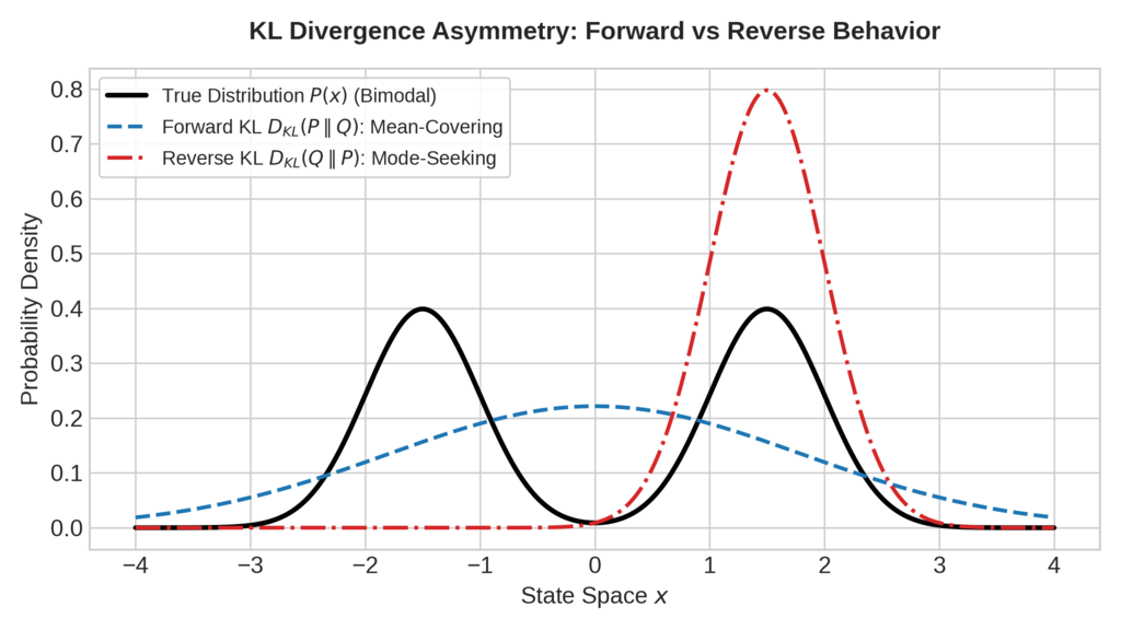
Forward KL: D_{\text{KL}}(P \parallel Q) (Zero-Avoiding / Mean-Covering)

D_{\text{KL}}(P \parallel Q) = \int p(x) \ln p(x) \, dx - \int p(x) \ln q(x) \, dx

If p(x) > 0 at some point x, q(x) must also be greater than 0. If q(x) \to 0 while p(x) > 0, the ratio \frac{p(x)}{q(x)} \to \infty, causing the divergence to explode to infinity. As a consequence, minimizing forward KL forces Q to stretch across all modes of P to avoid zero-density penalties, leading to mean-covering (broad) behavior.

Reverse KL: D_{\text{KL}}(Q \parallel P) (Zero-Forcing / Mode-Seeking)

D_{\text{KL}}(Q \parallel P) = \int q(x) \ln q(x) \, dx - \int q(x) \ln p(x) \, dx

Here, the expectation is taken with respect to model distribution Q. If p(x) = 0 in a region, Q(x) is forced to be exactly 0 to prevent the integral from exploding. When approximating a multi-modal distribution P, minimizing reverse KL causes Q to collapse into a single high-density mode of P, ignoring other modes entirely. This mode-seeking behavior forms the optimization basis for Variational Inference (VI) and Markov Decision Processes in Reinforcement Learning.

Decomposition of KL Divergence into Cross-Entropy Loss Functions

Using basic logarithmic properties, we can decompose KL divergence into two foundational information-theoretic terms:

D_{\text{KL}}(P \parallel Q) = \sum_{x \in \mathcal{X}} P(x) \log_2 \left( \frac{P(x)}{Q(x)} \right) = \sum_{x \in \mathcal{X}} P(x) \left[ \log_2 P(x) - \log_2 Q(x) \right]

D_{\text{KL}}(P \parallel Q) = \sum_{x \in \mathcal{X}} P(x) \log_2 P(x) - \sum_{x \in \mathcal{X}} P(x) \log_2 Q(x)

Recognizing that the first term is the negative Shannon entropy -H(P), and defining the second term as the Cross-Entropy H(P, Q):

H(P, Q) = -\sum_{x \in \mathcal{X}} P(x) \log_2 Q(x)

we obtain the structural relationship:

D_{\text{KL}}(P \parallel Q) = H(P, Q) - H(P)

\implies H(P, Q) = H(P) + D_{\text{KL}}(P \parallel Q)

Direct Machine Learning Implications

In supervised classification, the ground-truth distribution P is empirical and fixed (represented as one-hot label vectors). Because the target labels are constant throughout training, the intrinsic entropy H(P) is a fixed constant (H(P) = 0 for deterministic one-hot targets).

Therefore, minimizing the model’s cross-entropy loss function with respect to network parameters \theta is mathematically identical to minimizing the KL divergence D_{\text{KL}}(P \parallel Q_\theta):

\arg\min_{\theta} H(P, Q_\theta) \equiv \arg\min_{\theta} D_{\text{KL}}(P \parallel Q_\theta)

This proves that training deep learning classifiers via cross-entropy directly forces the model’s output probability distribution Q_\theta to match the true data-generating distribution P.

Multivariate Information Measures: Joint, Conditional, and Mutual Information

In real-world physical and computational systems, processes rarely exist in total isolation. When analyzing complex systems governed by multiple stochastic variables, single-variable Shannon entropy is insufficient. Information theory addresses multi-variable systems by introducing a unified framework composed of Joint Entropy, Conditional Entropy, and Mutual Information.

Joint Entropy and the Information Chain Rule

Let X and Y be two discrete random variables defined over alphabets \mathcal{X} and \mathcal{Y}, governed by a joint probability distribution p(x, y) = P(X = x, Y = y).

Definition

The Joint Entropy H(X, Y) quantifies the total combined uncertainty inherent in observing both random variables simultaneously:

H(X, Y) = -\sum_{x \in \mathcal{X}} \sum_{y \in \mathcal{Y}} p(x, y) \log_2 p(x, y) = \mathbb{E}_{(X,Y) \sim p}[-\log_2 p(X, Y)]

For continuous random variables with joint probability density function p(x, y), joint differential entropy is given by:

h(X, Y) = -\int_{-\infty}^{\infty} \int_{-\infty}^{\infty} p(x, y) \ln p(x, y) \, dx \, dy

The Chain Rule for Entropy

Using the probability chain rule p(x, y) = p(x) p(y|x) = p(y) p(x|y), we can decompose joint entropy into marginal and conditional components:

H(X, Y) = -\sum_{x \in \mathcal{X}} \sum_{y \in \mathcal{Y}} p(x, y) \log_2 \left[ p(x) p(y\vert{}x) \right]

H(X, Y) = -\sum_{x \in \mathcal{X}} \sum_{y \in \mathcal{Y}} p(x, y) \log_2 p(x) - \sum_{x \in \mathcal{X}} \sum_{y \in \mathcal{Y}} p(x, y) \log_2 p(y\vert{}x)

Noting that \sum_{y \in \mathcal{Y}} p(x, y) = p(x) (marginal probability), the first summation simplifies to:

-\sum_{x \in \mathcal{X}} p(x) \log_2 p(x) = H(X)

Defining the second summation as the Conditional Entropy H(Y|X), we arrive at the fundamental Chain Rule of Information:

H(X, Y) = H(X) + H(Y\vert{}X) = H(Y) + H(X\vert{}Y)

By induction, for a sequence of n random variables X_1, X_2, \dots, X_n, the general chain rule expands as:

H(X_1, X_2, \dots, X_n) = \sum_{i=1}^{n} H(X_i \mid X_1, \dots, X_{i-1})

Conditional Entropy (Equivocation)

Conditional Entropy H(Y|X) measures the average remaining uncertainty in variable Y after the outcome of variable X has been fully observed.

Formal Definition

H(Y\vert{}X) = \sum_{x \in \mathcal{X}} p(x) H(Y \mid X = x) = -\sum_{x \in \mathcal{X}} p(x) \sum_{y \in \mathcal{Y}} p(y\vert{}x) \log_2 p(y\vert{}x)

H(Y\vert{}X) = -\sum_{x \in \mathcal{X}} \sum_{y \in \mathcal{Y}} p(x, y) \log_2 p(y\vert{}x)

Properties and Independence Bounds

A) Conditioning Reduces Entropy (Information Never Hurts): Observing a random variable X can never increase the average uncertainty regarding Y:

H(Y\vert{}X) \le H(Y)

Equality H(Y|X) = H(Y) holds if and only if X and Y are statistically independent (p(x, y) = p(x)p(y)).

B) Deterministic Dependence: If Y is a deterministic function of X (Y = f(X)), then H(Y|X) = 0.

Mutual Information (MI)

Mutual Information I(X; Y) quantifies the total volume of shared information between two random variables. It measures the reduction in uncertainty of X brought about by observing Y (or vice versa).

Formal Definition via Log-Likelihood Ratios

I(X; Y) = \sum_{x \in \mathcal{X}} \sum_{y \in \mathcal{Y}} p(x, y) \log_2 \left( \frac{p(x, y)}{p(x) p(y)} \right)

In continuous domains governed by densities p(x, y), p(x), and p(y):

I(X; Y) = \int_{-\infty}^{\infty} \int_{-\infty}^{\infty} p(x, y) \ln \left( \frac{p(x, y)}{p(x) p(y)} \right) dx \, dy

Derivation of Entropic Identities

We can express mutual information directly in terms of relative entropy (KL divergence):

I(X; Y) = D_{\text{KL}}\big( p(x, y) \parallel p(x)p(y) \big)

Because KL divergence is non-negative (D_{\text{KL}} \ge 0), mutual information is strictly non-negative:

I(X; Y) \ge 0

Expanding the logarithm in the definition of I(X; Y):

I(X; Y) = \sum_{x} \sum_{y} p(x, y) \log_2 p(x, y) - \sum_{x} \sum_{y} p(x, y) \log_2 p(x) - \sum_{x} \sum_{y} p(x, y) \log_2 p(y)

I(X; Y) = -H(X, Y) + H(X) + H(Y)

Rearranging this identity yields the core relationship linking marginal, joint, conditional, and mutual information:

I(X; Y) = H(X) - H(X\vert{}Y)

I(X; Y) = H(Y) - H(Y\vert{}X)

I(X; Y) = H(X) + H(Y) - H(X, Y)

Summary of Multivariate Relationships

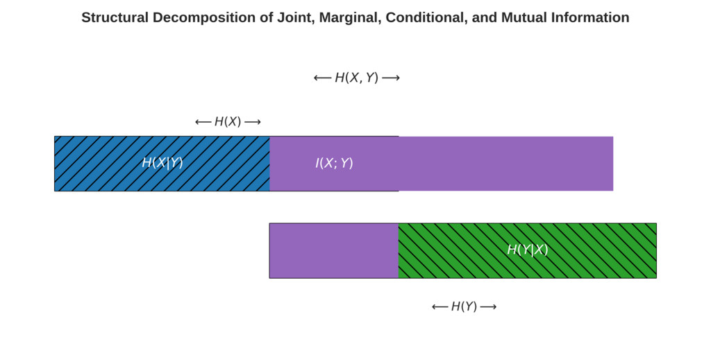
The exact interrelationships among all five fundamental information measures can be summarized through algebraic symmetries:

\begin{aligned} H(X, Y) &= H(X\vert{}Y) + I(X; Y) + H(Y\vert{}X) \\ H(X) &= H(X\vert{}Y) + I(X; Y) \\ H(Y) &= H(Y\vert{}X) + I(X; Y) \end{aligned}

When X and Y are completely independent, I(X; Y) = 0, causing joint entropy to equal the sum of marginals: H(X, Y) = H(X) + H(Y). When X and Y are deterministically identical (X = Y), I(X; X) = H(X), confirming that the mutual information of a variable with itself is simply its own Shannon entropy.

Advanced Principles: Minimum Mutual Information and Neural Bottlenecks

While the Principle of Maximum Entropy (MaxEnt) dictates how to assign probability distributions when facing complete or partial ignorance, representation learning in machine learning relies on dually constrained optimization frameworks. Two pivotal information-theoretic frameworks govern state-of-the-art representation learning: the Principle of Minimum Mutual Information (MinMI) and the Information Bottleneck (IB) Principle.

The Principle of Minimum Mutual Information (MinMI)

In high-dimensional feature extraction and self-supervised learning, extracting raw information is rarely sufficient; one must isolate task-relevant signals while stripping away nuisance attributes. This objective is formalized through the Principle of Minimum Mutual Information (MinMI).

Mathematical Formalization

Let X be an observed high-dimensional input signal (e.g., an image), Y be the target label or task objective, and Z = g(X) be a learned latent feature representation produced by a deterministic or stochastic encoding mapping g.

MinMI dictates that an optimal representation Z should minimize the mutual information I(X; Z) between the latent code Z and the raw input X, while enforcing structural constraints to preserve target information:

\min_{g} I(X; Z) \quad \text{subject to} \quad I(Z; Y) \ge I_{\text{target}}

Equivalence to Maximum Entropy under Known Marginals

A profound mathematical connection links MinMI to Jaynes’ MaxEnt principle. Recall the identity expanding mutual information in terms of entropy:

I(X; Z) = H(Z) - H(Z\vert{}X)

Suppose the encoder g(X) is a deterministic mapping. In a deterministic system, knowing X fully specifies Z, rendering the conditional entropy zero (H(Z|X) = 0). Under this condition, minimizing mutual information simplifies directly to minimizing latent entropy:

\min_{g} I(X; Z) \implies \min_{g} H(Z)

However, if the marginal distributions p(x) and p(y) are known and fixed prior conditions, minimizing the mutual information between latent features and irrelevant background noise is equivalent to maximizing the conditional entropy of the representation given the noise attributes. Thus, MinMI acts as a regularizer preventing the representation Z from memorizing instance-specific noise patterns.

The Information Bottleneck (IB) Principle

Formulated by Naftali Tishby, Fernando, and Bialek, the Information Bottleneck (IB) Principle extends MinMI into a variational framework that models deep neural network representations as information trade-off frontiers.

Markov Chain Structure of Deep Networks

Consider a deep neural network processing an input random variable X to predict a target random variable Y. The successive hidden layer activations T_1, T_2, \dots, T_L form a layered Markov chain:

Y \to X \to T_1 \to T_2 \to \dots \to T_L \to \hat{Y}

By the Data Processing Inequality (DPI), processing data through a cascade of stochastic or deterministic transformations cannot create new information. Consequently, mutual information monotonically decreases along the network depth:

I(X; Y) \ge I(T_1; Y) \ge I(T_2; Y) \ge \dots \ge I(T_L; Y)

I(Y; X) \ge I(X; T_1) \ge I(X; T_2) \ge \dots \ge I(X; T_L)

The Information Bottleneck Objective Function

The goal of an optimal bottleneck layer representation T is to act as a minimal sufficient statistic: it must compress X as much as possible while preserving maximum information about Y. This is formulated as a constrained optimization problem:

\max_{p(t\vert{}x)} I(Y; T) \quad \text{subject to} \quad I(X; T) \le R

where R denotes the maximum allowable information rate (complexity constraint). Using a Lagrange multiplier \beta \ge 0, we formulate the unconstrained Information Bottleneck Lagrangian:

\mathcal{L}_{\text{IB}}[p(t\vert{}x)] = I(Y; T) - \beta I(X; T)

Operational interpretation of the hyperparameter \beta:

• \beta \to 0: The network prioritizes maximum compression (I(X; T) \to 0), disregarding prediction error.
• \beta \to \infty: The network prioritizes maximum target prediction (I(Y; T) \to I(X;Y)), allocating unlimited capacity to store input details.

Analytical Solution of the IB Self-Consistent Equations

To find the optimal stochastic mapping p(t|x) that maximizes \mathcal{L}_{\text{IB}}, we take the functional derivative of the Lagrangian with respect to p(t|x) and set it to zero under normalization constraints \sum_t p(t|x) = 1.

This yields the set of Tishby IB self-consistent equations:

p(t\vert{}x) = \frac{p(t)}{Z(x, \beta)} \exp\left( -\beta D_{\text{KL}}\big( p(y\vert{}x) \parallel p(y\vert{}t) \big) \right)

where Z(x, \beta) is the normalizing partition function:

Z(x, \beta) = \sum_{t} p(t) \exp\left( -\beta D_{\text{KL}}\big( p(y\vert{}x) \parallel p(y\vert{}t) \big) \right)

and the marginal representations update iteratively via:

p(t) = \sum_{x} p(x) p(t\vert{}x)

p(y\vert{}t) = \frac{1}{p(t)} \sum_{x} p(x, y) p(t\vert{}x)

This analytical solution demonstrates that the optimal stochastic assignment p(t|x) decays exponentially with the KL divergence between the target conditional distribution given the input p(y|x) and the target distribution given the latent representation p(y|t).

Deep Learning Training Dynamics: Fitting vs. Compression Phases

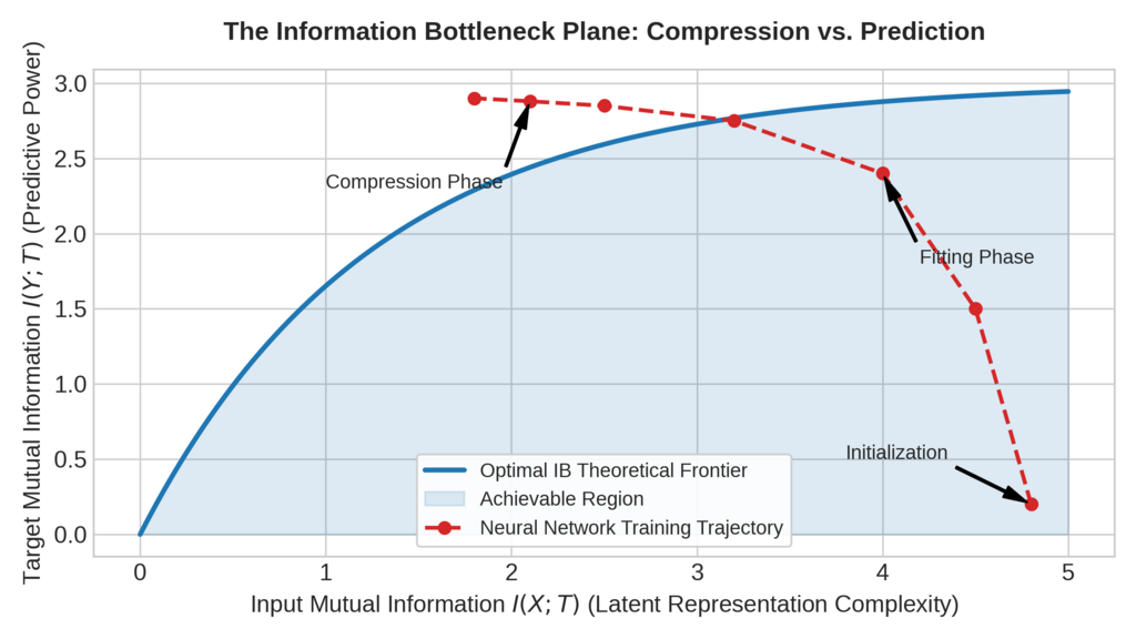
By projecting deep neural network training trajectories onto the Information Bottleneck Plane (plotting I(X; T) on the horizontal axis and I(Y; T) on the vertical axis), Tishby and Schwartz uncovered two distinct phases of Stochastic Gradient Descent (SGD) optimization:

The Empirical Fitting Phase (Fast)

In the early epochs of training, gradient updates are dominated by high mean signal components. The network rapidly increases I(Y; T) to improve classification accuracy. Simultaneously, I(X; T) increases as the network memorizes input features, moving upward and rightward in the IB plane.

The Information Compression Phase (Slow)

In later epochs, the mean gradient magnitudes shrink relative to the stochastic noise introduced by mini-batch sampling. The SGD dynamics behave like an implicit diffusion process governed by a Fokker-Planck equation. This stochastic noise forces the network representation T to compress input details, reducing I(X; T) while preserving predictive power I(Y; T). During this phase, the representation trajectory moves leftward along the optimal theoretical IB frontier, explaining why deep networks generalize well despite overparameterization.

Physical Analogies and Quantum Mechanics

The bridge connecting information-theoretic entropy to physical science is deep, historically foundational, and mathematically robust. As noted by John von Neumann during the conceptualization of Shannon’s theory, the mathematics governing information uncertainty shares an exact isomorphism with statistical mechanics and quantum physics.

Statistical Mechanics and Boltzmann’s Entropy

In 1877, Ludwig Boltzmann formulated the statistical interpretation of thermodynamic entropy, establishing that macroscopic physical properties arise from microscopic atomic configurations. This relationship is immortalized by the Boltzmann-Planck equation:

S = k_B \ln W

where S is the thermodynamic entropy, k_B = 1.380649 \times 10^{-23} , \text{J/K} is the Boltzmann constant, and W represents the number of real microstates (positions and momenta of atoms) corresponding to a given macroscopic thermodynamic state.

The Second Law and Universal Thermal Death

In an isolated thermodynamic system, spontaneous irreversible processes drive the system toward maximum entropy, leveling out energy and temperature gradients until equilibrium is attained. If this macroscopic principle is extrapolated to the entire universe as an adiabatic isolated system, it leads to the theoretical conjecture of heat death (entropic death), where no free energy gradients remain to power physical work—mirroring how maximum Shannon entropy corresponds to complete statistical uniformity where no predictive signal survives.

Entropic Formulations of the Heisenberg Uncertainty Principle

Beyond thermodynamics, information entropy governs fundamental quantum mechanical limits. The standard Heisenberg Uncertainty Principle states that pairs of conjugate physical observables (such as position x and momentum p_x) cannot simultaneously be measured with arbitrary precision:

\Delta x \Delta p_x \ge \frac{\hbar}{2}

However, standard deviation-based uncertainty bounds fail for multi-modal quantum wave functions. To resolve this, physicists including Hirschman, Beckner, and Bialynicki-Birula formulated the Entropic Uncertainty Principle, which replaces standard deviations with differential entropies.

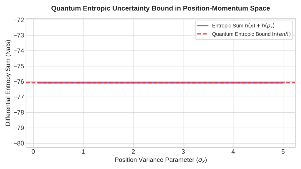
Let \psi(x) be a normalized position-space wave function, and let \tilde{\psi}(p_x) be its Fourier transform representing the momentum-space wave function. The differential entropies of their respective probability density distributions satisfy the strict lower bound:

h(x) + h(p_x) \ge \ln(e \pi \hbar)

where \hbar = \frac{h}{2\pi} is the reduced Planck constant.

Deriving Heisenberg’s Limit from Maximum Entropy

Because the differential entropy of a Gaussian distribution acts as the absolute upper bound among all probability densities with identical variance, we can substitute the Gaussian entropy limit h(z) \le \frac{1}{2}\ln(2\pi e \sigma_z^2) into the entropic sum:

\frac{1}{2}\ln(2\pi e \sigma_x^2) + \frac{1}{2}\ln(2\pi e \sigma_{p_x}^2) \ge \ln(e \pi \hbar)

Exponentiating both sides yields the product of variances:

2\pi e \sigma_x \sigma_{p_x} \ge e \pi \hbar \implies \sigma_x \sigma_{p_x} \ge \frac{\hbar}{2}

This proves that quantum indeterminacy is fundamentally an information-theoretic limitation rather than an artifact of imperfect measurement instrumentation.

Data Compression and Source Coding Theorems

One of the most profound practical applications of Shannon’s information theory lies in data compression. To transmit symbols from an information source S across a communication channel efficiently, symbols are mapped into binary codewords. The fundamental limits governing how compact these encodings can be are established by Shannon’s Source Coding Theorems.

Shannon’s First Theorem (Source Coding Theorem)

Shannon’s First Theorem establishes an absolute mathematical boundary on lossless data compression: it is impossible to represent the outputs of a stationary information source S using a source code whose average codeword length L is strictly less than the source entropy H(S):

H(S) \le L < H(S) + 1

Mathematical Formulation of Average Codeword Length

Let an information source emit symbols s_i from an alphabet of size N, where each symbol occurs with probability p_i. If a coding scheme assigns a binary codeword of integer length l_i to each symbol s_i, the expected average codeword length L per symbol is defined as:

$$L = \sum_{i=1}^{N} p_i l_i$$

The Source Coding Theorem guarantees that L can be made arbitrarily close to the source entropy H(S) (measured in bits) by encoding blocks of symbols jointly, but it can never breach the entropic barrier without incurring data loss.

Prefix Codes and the Kraft-McMillan Inequality

To ensure that compressed bitstreams can be decoded unambiguously without requiring explicit delimiters or separator characters, modern coding algorithms utilize prefix codes (instantaneous codes). A prefix code satisfies the prefix condition: no codeword is a prefix of any other codeword in the codebook.

The Kraft-McMillan Inequality

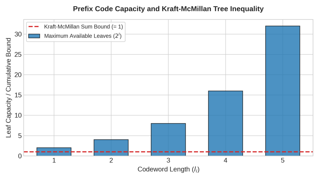
The structural feasibility of constructing prefix codes with specific codeword lengths l_1, l_2, \dots, l_N over a binary alphabet is governed by the Kraft-McMillan inequality:

\sum_{i=1}^{N} 2^{-l_i} \le 1

If a set of integer lengths satisfies this inequality, a uniquely decodable prefix code (such as a Huffman tree) can be constructed. Conversely, any uniquely decodable code must satisfy the inequality.

Proof Outline via Binary Code Trees

Geometrically, binary prefix codes can be visualized as leaf nodes on a binary tree of maximum depth equal to the maximum codeword length l_{\max}. Each chosen codeword of length l_i consumes a fraction 2^{-l_i} of the total available leaf capacity of the binary tree. Because the total capacity of a binary tree of depth l_{\max} cannot exceed 1, the sum of all fractions allocated by the codewords must be less than or equal to unity, directly proving the inequality.

Code Efficiency and Asymptotic Optimality

We define coding efficiency \eta as the ratio of source entropy to average codeword length:

\eta = \frac{H(S)}{L}

When every symbol’s probability matches an exact negative power of two such that p_i = 2^{-l_i}, Huffman coding achieves an average length L = H(S), resulting in \eta = 100% efficiency. When probabilities do not align cleanly with powers of two, extending the source alphabet to block groupings n allows block codes (such as Shannon-Fano-Elias or arithmetic coding) to approach the entropy limit asymptotically:

\lim_{n \to \infty} \frac{L_n}{n} = H(S)

This guarantees that high-entropy sources are inherently incompressible, while low-entropy sources containing high redundancy possess immense compression potential.

Conclusion

Entropy has evolved far beyond its origins in 19th-century statistical mechanics and mid-20th-century telecommunication engineering. What began as Ludwig Boltzmann’s probabilistic measure of physical disorder and Claude Shannon’s formal quantification of communication uncertainty has matured into a foundational mathematical language that underpins nearly every major discipline in computer science and artificial intelligence. By bridging discrete combinatorial counting, continuous probability spaces, physical thermodynamic limits, and quantum mechanics, entropy provides a universal lens through which we measure, compress, and optimize information.

In contemporary technological applications, the influence of entropy is both pervasive and indispensable. In data transmission and storage systems, Shannon’s source coding theorems and prefix code limits dictate how massive multimedia streams, encrypted archives, and cloud databases are compressed without losing a single bit of fidelity. In modern machine learning and deep learning, cross-entropy loss functions and Kullback-Leibler divergences serve as the primary optimization engines driving state-of-the-art neural network classifiers, large language models, and variational generative architectures. Furthermore, advanced principles like the Information Bottleneck framework reveal how deep neural networks intelligently discard irrelevant nuisance noise while preserving critical predictive features during stochastic gradient descent training.

As computer science ventures further into high-performance computing, complex neural architectures, and quantum information processing, entropy remains our most reliable compass for navigating uncertainty. Whether calculating the capacity limits of emerging communication channels or bounding quantum states through entropic uncertainty relations, mastering entropy is essential for anyone seeking to push the boundaries of computational theory. We invite you to explore these interconnected mathematical frameworks further, apply them to your own system designs, and discover how quantifying uncertainty can unlock unprecedented computational efficiency.

Bibliography

1. Shannon, C. E. (1948). A Mathematical Theory of Communication. The Bell System Technical Journal, 27(3), 379–423.
2. Boltzmann, L. (1877). Über die Beziehung zwischen dem zweiten Hauptsatze der mechanischen Wärmetheorie und der Wahrscheinlichkeitsrechnung respektive den Sätzen über das Wärmegleichgewicht. Wiener Berichte, 76, 373–435.
3. Jaynes, E. T. (1957). Information Theory and Statistical Mechanics. Physical Review, 106(4), 620–630.
4. Kullback, S., & Leibler, R. A. (1951). On Information and Sufficiency. The Annals of Mathematical Statistics, 22(1), 79–86.
5. Cover, T. M., & Thomas, J. A. (2006). Elements of Information Theory (2nd ed.). Wiley-Interscience.
6. Tishby, N., Pereira, F. C., & Bialek, W. (2000). The Information Bottleneck Method. Proceedings of the 37th Annual Allerton Conference on Communication, Control, and Computing, 368–377.
7. Tishby, N., & Zaslavsky, N. (2015). Deep Learning and the Information Bottleneck Principle. IEEE Information Theory Workshop (ITW), 1–5.
8. Hirschman, I. I. (1957). A Note on Entropy. Proceedings of the National Academy of Sciences, 43(6), 447–449.
9. Bialynicki-Birula, I., & Mycielski, J. (1975). Uncertainty Relations for Information Entropy in Wave Mechanics. Communications in Mathematical Physics, 44(2), 129–132.
10. MacKay, D. J. C. (2003). Information Theory, Inference and Learning Algorithms. Cambridge University Press.