 Francisco Yepes Barrera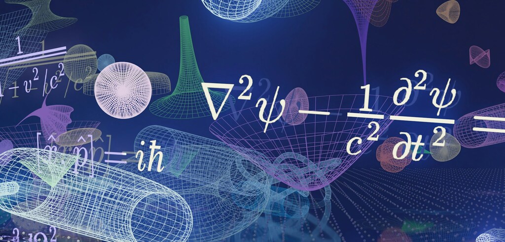
Brecht Corbeel - https://unsplash.com/photos/quantum-physics-equations-and-abstract-wireframe-shapes-on-blue-background-Z8s6ea-60cg
Table of Contents
What is Quantum Mechanics?
Definition and Scope
Quantum Mechanics (QM) is the fundamental theoretical framework of modern physics designed to describe the behavior of matter and radiation at atomic and subatomic scales (typically at length scales below 10^{-9}\text{ m}).
While classical mechanics (Newtonian and Lagrangian) relies on a deterministic and continuous view of the universe—where the state of a system is uniquely defined by position coordinates q_i and momentum p_i in phase space—quantum mechanics replaces this determinism with a probabilistic and discrete mathematical description.
The defining hallmark of QM is quantization: physical quantities (such as energy, angular momentum, or electric charge) cannot take arbitrary continuous values but are constrained to a discrete spectrum of allowed values (quanta).
Historical Evolution & Key Pioneers
The formulation of quantum mechanics arose from the failure of classical physics to explain several experimental anomalies at the turn of the 20th century.
1. The Ultraviolet Catastrophe and Blackbody Radiation (Max Planck, 1900)
Classical electromagnetism (the Rayleigh-Jeans law) predicted that an ideal blackbody would emit an infinite amount of radiant energy at high frequencies (the ultraviolet region), violating the principle of conservation of energy. Max Planck resolved this crisis by hypothesizing that atomic oscillators in the cavity walls exchange energy with the electromagnetic field only in discrete packets (E = n h \nu, with n \in \mathbb{N} and h \approx 6.626 \times 10^{-34} \text{ J}\cdot\text{s}).
2. The Photoelectric Effect and Photons (Albert Einstein, 1905)
Einstein extended Planck’s hypothesis by showing that quantization is not merely a boundary property of atomic oscillators but an intrinsic property of electromagnetic radiation itself. Light consists of quanta of energy (later named photons), each carrying energy and momentum:
E = \hbar \omega, \quad \vec{p} = \hbar \vec{k}where \hbar = \frac{h}{2\pi} is the reduced Planck constant, \omega is the angular frequency, and \vec{k} is the wave vector.
3. The Bohr Model of the Atom (Niels Bohr, 1913)
Bohr explained the discrete emission spectrum of the hydrogen atom by postulating that electrons orbit the nucleus only along stationary quantized orbits where angular momentum L is an integer multiple of \hbar:
L = n\hbar \quad (n = 1, 2, 3, \dots)
4. De Broglie’s Hypothesis (Louis de Broglie, 1924)
De Broglie generalized the wave-particle duality of light by proposing that ordinary matter (such as electrons) also possesses wave-like nature. A particle with momentum p has an associated wavelength:
\lambda = \frac{h}{p}5. Matrix Mechanics and Wave Mechanics (1925–1926)
- Werner Heisenberg (1925): Formulated matrix mechanics, eliminating unobservable electron orbits and describing physical observables using infinite-dimensional matrices and non-commutative algebraic equations.
- Erwin Schrödinger (1926): Developed wave mechanics, introducing a partial differential equation based on the wave function \psi(\vec{r},t).
- Paul Dirac & John von Neumann (1930): Proved the mathematical equivalence between Heisenberg’s and Schrödinger’s formulations, unifying the theory within the abstract framework of Hilbert spaces.
Key Concepts & Mathematical Formalism
Hilbert Space Formalism & Bra-Ket Notation
The rigorous mathematical language of quantum mechanics rests on complex Hilbert spaces \mathcal{H} equipped with a positive-definite inner product.
1. State Vectors (Kets and Bras)
- Ket (\vert{}\psi\rangle): Represents a quantum state. It is a complex column vector belonging to the space \mathcal{H}.
- Bra (\langle\psi\vert{}): A row vector (the conjugate transpose) belonging to the dual space \mathcal{H}^*. Mathematically: \langle\psi\vert{} = (\vert{}\psi\rangle)^\dagger.
- Inner Product: Given two states \vert{}\phi\rangle and \vert{}\psi\rangle, their inner product \langle\phi\vert{}\psi\rangle \in \mathbb{C} represents the probability amplitude. A physically admissible state vector must be normalized:
\langle\psi\vert{}\psi\rangle = 12. Operators and Observables
Physical observables (such as position, momentum, spin, and energy) are represented by Hermitian linear operators\hat{A} acting on elements of \mathcal{H}.
An operator is Hermitian if it equals its adjoint (\hat{A}^\dagger = \hat{A}), guaranteeing two essential properties:
- All eigenvalues \alpha_n in the eigenvalue equation \hat{A}\vert{}\alpha_n\rangle = \alpha_n \vert{}\alpha_n\rangle are real numbers (representing physical measurement outcomes).
- Eigenvectors \vert{}\alpha_n\rangle corresponding to distinct eigenvalues form a complete orthonormal basis of the Hilbert space:
\langle\alpha_n\vert{}\alpha_m\rangle = \delta_{nm}, \quad \sum_n \vert{}\alpha_n\rangle\langle\alpha_n\vert{} = \hat{\mathbb{I}}Inner Product vs. Outer Product in Dirac Notation
In Dirac notation, placing a bra and a ket in different relative positions yields two distinct mathematical operations with complementary physical meanings:
| Property | Inner Product | Outer Product |
| Syntax | \langle\phi\vert{}\psi\rangle | \vert{}\psi\rangle\langle\phi\vert |
| Object Type | Complex number (Scalar \mathbb{C}) | Linear Operator (Matrix) |
| Mapping | \mathcal{H} \times \mathcal{H} \to \mathbb{C} | \mathcal{H} \to \mathcal{H} |
| Physical Meaning | Probability amplitude / Overlap | Projection / State transformation |
1. Inner Product: \langle\phi\vert{}\psi\rangle
- Mathematical Nature: The inner product pairs a bra on the left and a ket on the right, yielding a complex scalar (\mathbb{C}).
- Matrix Form: Product of a 1 \times N row vector (conjugate transpose) and an N \times 1 column vector:
\langle\phi\vert{}\psi\rangle = \begin{pmatrix} \phi_1^* & \phi_2^* & \cdots & \phi_N^* \end{pmatrix} \begin{pmatrix} \psi_1 \\ \psi_2 \\ \vdots \\ \psi_N \end{pmatrix} = \sum_{i=1}^N \phi_i^* \psi_i \quad \in \mathbb{C}- Physical Significance: Yields the overlap probability amplitude. The absolute square \vert{}\langle\phi\vert{}\psi\rangle\vert{}^2 gives the probability of finding the system in state \vert{}\phi\rangle upon measurement when prepared in \vert{}\psi\rangle.
2. Outer Product: \vert{}\psi\rangle\langle\phi\vert{}
- Mathematical Nature: The outer product pairs a ket on the left and a bra on the right, producing an N \times N matrix (a linear operator).
- Matrix Form: Product of an N \times 1 column vector and a 1 \times N row vector:
\vert{}\psi\rangle\langle\phi\vert{} = \begin{pmatrix} \psi_1 \\ \psi_2 \\ \vdots \\ \psi_N \end{pmatrix} \begin{pmatrix} \phi_1^* & \phi_2^* & \cdots & \phi_N^* \end{pmatrix} = \begin{pmatrix} \psi_1 \phi_1^* & \psi_1 \phi_2^* & \cdots & \psi_1 \phi_N^* \\ \psi_2 \phi_1^* & \psi_2 \phi_2^* & \cdots & \psi_2 \phi_N^* \\ \vdots & \vdots & \ddots & \vdots \\ \psi_N \phi_1^* & \psi_N \phi_2^* & \cdots & \psi_N \phi_N^* \end{pmatrix}- Projection Operators: When ket and bra use the same orthonormal state \vert{}\phi_n\rangle, it forms a projection operator \hat{P}_n = \vert{}\phi_n\rangle\langle\phi_n\vert{}, projecting any vector onto that basis state.
\sum_{n} \vert{}\phi_n\rangle\langle\phi_n\vert{} = \hat{\mathbb{I}}- Spectral Decomposition: Any Hermitian operator \hat{A} can be expressed in terms of outer products of its eigenvectors weighted by its eigenvalues:
\hat{A} = \sum_{n} \alpha_n \vert{}\alpha_n\rangle\langle\alpha_n\vert{}- Density Matrix (Mixed States): Describes statistical ensembles or open quantum systems via the density operator:
\hat{\rho} = \sum_{i} p_i \vert{}\psi_i\rangle\langle\psi_i\vert{}Fundamental Postulates and Quantum Phenomena
1. Superposition Principle
If \vert{}\psi_1\rangle and \vert{}\psi_2\rangle are valid states of a system, any linear combination:
\vert{}\Psi\rangle = c_1 \vert{}\psi_1\rangle + c_2 \vert{}\psi_2\rangle \quad (c_1, c_2 \in \mathbb{C})is also a valid physical state, provided it is normalized: \vert{}c_1\vert{}^2 + \vert{}c_2\vert{}^2 = 1.
Born’s Rule: Measuring an observable \hat{A} on a system in state \vert{}\Psi\rangle yields eigenvalue \alpha_i (associated with eigenstate \vert{}\psi_i\rangle) with probability:
P(\alpha_i) = \vert{}\langle\psi_i\vert{}\Psi\rangle\vert{}^2 = \vert{}c_i\vert{}^22. Quantum Measurement & Wave Function Collapse
Measurement in quantum mechanics is a non-unitary, probabilistic process. Upon measuring an observable \hat{A} and obtaining outcome \alpha_i, the state vector instantly projects onto the corresponding eigenstate:
\vert{}\Psi\rangle \xrightarrow{\text{Measurement of } \alpha_i} \vert{}\psi_i\rangleThis phenomenon is known as the collapse of the wave function.
3. Heisenberg’s Uncertainty Principle
Observables represented by non-commuting operators ([\hat{A}, \hat{B}] = \hat{A}\hat{B} - \hat{B}\hat{A} \neq 0) cannot be simultaneously measured with arbitrary precision.
The Robertson-Heisenberg uncertainty relation states:
\sigma_A \sigma_B \ge \frac{1}{2} \left\vert{} \langle [\hat{A}, \hat{B}] \rangle \right\vert{}For the position operator \hat{x} and momentum operator \hat{p}_x = -i\hbar \frac{\partial}{\partial x}, the canonical commutation relation [\hat{x}, \hat{p}_x] = i\hbar gives:
\Delta x \cdot \Delta p_x \ge \frac{\hbar}{2}4. Time Evolution: The Schrödinger Equation
The continuous, deterministic, and unitary time evolution of a non-relativistic quantum state is governed by the time-dependent Schrödinger equation:
i\hbar \frac{\partial}{\partial t} \vert{}\psi(t)\rangle = \hat{H} \vert{}\psi(t)\ranglewhere \hat{H} is the Hamiltonian operator (total energy of the system).
In position space (\psi(\vec{r},t) = \langle \vec{r} \vert{} \psi(t) \rangle), for a particle of mass m in a potential V(\vec{r},t):
i\hbar \frac{\partial \psi(\vec{r},t)}{\partial t} = \left( -\frac{\hbar^2}{2m} \nabla^2 + V(\vec{r},t) \right) \psi(\vec{r},t)Quantum Entanglement and Bell’s Theorem
1. Mathematical Definition of Entanglement
Consider a composite system consisting of two subsystems and B, associated with Hilbert spaces \mathcal{H}_A and \mathcal{H}_B. The total Hilbert space is the tensor product \mathcal{H} = \mathcal{H}_A \otimes \mathcal{H}_B.
- Separable State: A state is separable if it can be written as a product of single-particle states:
\vert{}\Psi_{AB}\rangle = \vert{}\psi_A\rangle \otimes \vert{}\psi_B\rangle- Entangled State: A state is entangled if it cannot be factored into individual subsystem states.
A classic example is the Bell singlet state for two spin-1/2 particles:
\vert{}\Psi^-\rangle = \frac{1}{\sqrt{2}} \left( \vert{}{\uparrow}_A\rangle \vert{}{\downarrow}_B\rangle - \vert{}{\downarrow}_A\rangle \vert{}{\uparrow}_B\rangle \right)2. The EPR Paradox (1935) and Local Hidden Variables
To avoid instantaneous collapse that seemed to violate relativistic causality, Einstein, Podolsky, and Rosen (EPR) argued that quantum mechanics was incomplete. They proposed the existence of local hidden variables (\lambda)—pre-existing properties determined at particle creation—so that no instantaneous action-at-a-distance was needed.
3. Bell’s Theorem and Inequality (1964)
John Stewart Bell showed that EPR’s assumption of local realism (realism: physical properties exist independent of measurement; locality: no influence travels faster than light) leads to strict mathematical limits on statistical correlations between distant measurements.
The CHSH form of Bell’s Inequality dictates that under any local realistic theory:
\vert{}S_{\text{CHSH}}\vert{} = \vert{}E(a,b) - E(a,c) + E(d,b) + E(d,c)\vert{} \le 24. Experimental Violation and Significance
Quantum mechanical calculations predict a maximum violation up to Cirel’son’s bound:
S_{\text{CHSH}}^{\text{quantum}} = 2\sqrt{2} \approx 2.828 > 2Experiments pioneered by Alain Aspect (1982) and refined to loophole-free tests in 2015 (awarded the 2022 Nobel Prize in Physics to Aspect, Clauser, and Zeilinger) conclusively proved that Bell’s inequalities are violated.
Physical Consequences:
- Nature violates Local Realism: Particles do not hold predetermined values before measurement.
- Quantum Non-locality: Measuring particle A instantly collapses the state of B, regardless of physical distance.
- No-Signaling Theorem: This non-locality cannot be used for faster-than-light communication. Because measurement outcomes at A are fundamentally random, observer sees only noise until receiving A‘s results via a classical channel bounded by the speed of light c.
Significance of Quantum Mechanics in Modern Science & Technology
The First Quantum Revolution
The early 20th century understanding of quantum principles yielded key foundational technologies:
- Semiconductor Physics: Understanding energy band structures in crystalline lattices (via Schrödinger’s equation in periodic potentials) enabled microprocessors, transistors, and diodes.
- Laser Technology: Based on Einstein’s 1917 theory of stimulated emission, powering optical fibers and medical technologies.
- Nuclear Magnetic Resonance (NMR/MRI): Utilizes radiofrequency fields manipulating nuclear spins in magnetic fields for non-invasive medical imaging.
The Second Quantum Revolution
Today’s quantum revolution focuses on manipulating and entangling individual quantum systems (single photons, trapped ions, superconducting qubits).
1. Quantum Computing
Unlike classical bits (0 or 1), qubits exist in superpositions:
\vert{}\psi\rangle = \alpha \vert{}0\rangle + \beta \vert{}1\rangle \quad (\alpha, \beta \in \mathbb{C}, \, \vert{}\alpha\vert{}^2 + \vert{}\beta\vert{}^2 = 1)- Quantum Parallelism: N qubits in superposition can represent 2^N states simultaneously.
- Quantum Speedup:
- Shor’s Algorithm: Factors large integers in polynomial time O((\log N)^3), challenging classical RSA encryption.
- Grover’s Algorithm: Offers a quadratic speedup O(\sqrt{N}) for searching unstructured databases.
2. Quantum Key Distribution (QKD)
Protocols like BB84 allow two parties (Alice and Bob) to generate a provably secure key based on fundamental physics:
- No-Cloning Theorem: Unknown quantum states cannot be duplicated.
- Observer Effect: Eavesdropping disturbs the quantum states, immediately alerting Alice and Bob to the intrusion.
3. Quantum Sensing and Metrology
- Atomic Clocks: Measure atomic transition frequencies with extreme stability, achieving precision under 1 second of drift per billion years.
- Atom Interferometry: Uses matter-wave interference for gravimetry and precise inertial navigation.
Bibliography
- Susskind, L., & Friedman, A. (2014). Quantum Mechanics: The Theoretical Minimum.
- Feynman, R. P., Leighton, R. B., & Sands, M. (2011). The Feynman Lectures on Physics, Vol. III: Quantum Mechanics.
- Griffiths, D. J., & Schroeter, D. F. (2018). Introduction to Quantum Mechanics (3rd ed.). Cambridge University Press.
- Sakurai, J. J., & Napolitano, J. (2020). Modern Quantum Mechanics (3rd ed.). Cambridge University Press.
- Nielsen, M. A., & Chuang, I. L. (2010). Quantum Computation and Quantum Information. Cambridge University Press.
- Einstein, A., Podolsky, B., & Rosen, N. (1935). Can quantum-mechanical description of physical reality be considered complete? Physical Review, 47(10), 777–780. https://doi.org/10.1103/PhysRev.47.777