 Francisco Yepes Barrera

Adlan - https://unsplash.com/photos/a-chess-board-with-a-chessboard-GYh9EwLAZC0
Table of Contents
Introduction
NNUE (Efficiently Updatable Neural Networks) is a specialized neural network architecture designed specifically to replace traditional handcrafted evaluation functions in alpha-beta search chess and shogi engines (such as Stockfish and YaneuraOu).
Invented by Yu Nasu in 2018 for computer shogi (drawing conceptual inspiration from Kunihito Hoki’s “Bonanza method” piece-square tables indexed by king location), NNUE solved a fundamental dilemma in game AI: deep neural networks (like AlphaZero or Leela Chess Zero) offer exceptional positional understanding but require massive GPU/TPU acceleration and slow down node evaluation speeds in traditional search trees. NNUE achieves deep-learning-grade evaluation accuracy while running entirely on commodity CPUs at speeds fast enough for millions of evaluations per second.
Foundations and Genesis of NNUE
The Classic Trade-Off in Tree Search
In game-tree search algorithms—such as Minimax variants, Principal Variation Search (PVS), and Alpha-Beta pruning—the effective search depth d is bound by the evaluation time per node t_{\text{eval}}. The total search time T_{\text{search}} for a branching factor b scales as:
T_{\text{search}} \propto b^d \cdot t_{\text{eval}}Classical chess engines relied on handcrafted evaluation functions (HCEs). These were explicit, linear (or shallow non-linear) combinations of material imbalances, piece-square tables, mobility metrics, and king safety terms:
f_{\text{HCE}}(s) = \sum_{k} w_k \cdot \phi_k(s)While computationally trivial to execute (yielding sub-microsecond evaluation times allowing millions of nodes per second), HCEs lacked deep positional understanding.
Conversely, deep neural network approaches popularized by AlphaZero and Leela Chess Zero utilize deep residual convolutional or transformer networks to evaluate board states s \in \mathcal{S}. While providing exceptional positional judgment, their raw forward-propagation latency (FP32/FP16 matrix multiplications across millions of parameters) is orders of magnitude too slow for commodity CPU-based alpha-beta engines, collapsing search throughput.
Historical Evolution: From Piece-Square Tables to NNUE
The architectural lineage of NNUE bridges this gap through three key milestones:
- Piece-Square Tables (PSTs): Standard positional evaluation maps piece types and board coordinates to scalar values. For a board state s, the score is an accumulation of static table lookups.
- The Bonanza Method (Kunihito Hoki, 2005): Developed for computer shogi, Bonanza generalized PSTs by treating evaluation weights as linear parameters trained via logistic regression on large databases of professional games. The score was computed as a linear dot product between a sparse binary feature vector x and a weight vector W: f(x) = W^T x. Because the feature vector was binary and sparse, updates during move execution required only adding/subtracting weights corresponding to changed pieces.
- NNUE (Yu Nasu, 2018): Nasu recognized that while a linear model is fast, it lacks non-linear abstraction. By inserting a non-linear neural network layer immediately after the sparse input layer—while preserving the incremental update property of sparse linear models—he created Efficiently Updatable Neural Networks.
Formal Problem Definition
Let \mathcal{S} be the set of all legal board states in a finite, zero-sum, perfect-information board game. We seek an evaluation function f_\theta: \mathcal{S} \to \mathbb{R} parameterized by weights \theta such that:
f_\theta(s) \approx v^*(s)
Where v^*(s) represents the true minimax game-theoretic value of state s (mapped to a normalized win-probability or centipawn scale).
To integrate seamlessly into alpha-beta search without hardware acceleration (GPUs/TPUs), f_\theta must satisfy two conflicting constraints:
- Representational Power: Capture complex long-range tactical and strategic interactions (pawn chains, king vulnerability, spatial control).
- Incremental Computational Complexity: The evaluation delta when transitioning from state s_t to s_{t+1} via move m must execute in O(1) time regarding the total number of board features d, bypassing full-network forward passes at leaf nodes.
Evolution of NNUE Topologies Over Time
Before examining how subsequent layers process data, it is crucial to map how the NNUE architecture itself has evolved across generations of game engine research. Because incremental updates constrain the first layer to be a sparse linear transformation, architectural innovation has focused on modifying feature definitions, perspective merging, and hidden layer topologies.
Shogi HalfKP (The Origin, 2018)
Introduced by Yu Nasu for computer shogi, the original HalfKP architecture defined features entirely around the perspective of a single player’s king. In shogi, piece drops and dense board interactions make king safety paramount.
- Input Features: \text{King Square} \times \text{Piece Type} \times \text{Piece Square}.
- Topology: A single half-network accumulator (dimension h = 256) feeding into small fully connected dense layers (
256 -> 32 -> 32 -> 1).
Western Chess Adaptation: Dual-Perspective HalfKP (2020)
When ported to Western chess, the rules differ drastically (no piece drops, different mobility). Chess requires evaluating the position from both sides simultaneously because initiative and king safety apply to both players.
- Topology Modification: The network split into two identical subnets—one tracking White’s perspective relative to the White king, and one tracking Black’s perspective relative to the Black king.
- Dimension Scaling: Initial chess networks utilized
256 x 2accumulators feeding into concatenated dense layers.
HalfKAv2 and King Bucketing
As training sets grew, standard HalfKP suffered from data sparsity in rare king positions. HalfKAv2 introduced refined feature granularity (incorporating additional attack/defense interactions and more precise piece-square pairings) alongside King Bucketing.
Instead of maintaining separate weight vectors for all 64 individual king squares, king positions were clustered into spatial zones (buckets, e.g., K = 16 or 32). This allowed the network to share statistical weights across structurally similar king shelters (e.g., castled positions on the kingside vs. queenside) while drastically reducing memory overhead.
Modern Multi-Layer and Wider Configurations
Recent iterations in engines like Stockfish have scaled network widths and depths significantly (e.g., accumulator widths of h = 512 or 768 per perspective, feeding into wider hidden layers like 16 or 32 or 64 nodes, with multi-stage clipped activation functions). These larger networks balance inference latency against non-linear expressive capacity, achieving elite-level positional evaluation while maintaining sub-microsecond execution speeds.
Detailed Architectural Breakdown of NNUE
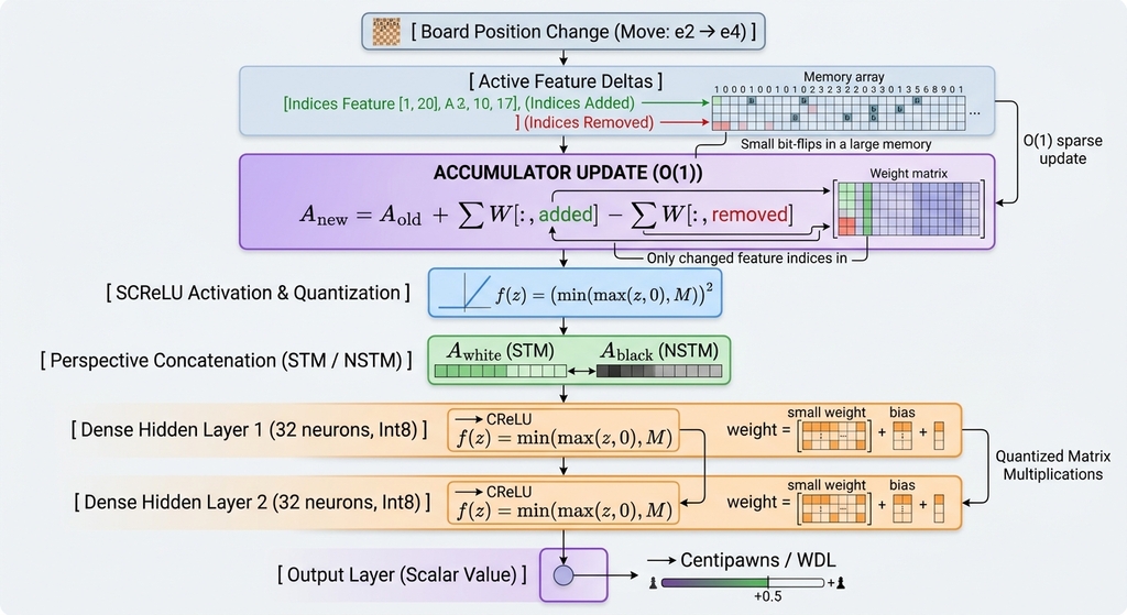
To understand how NNUE achieves its unique balance of deep neural network expressiveness and microsecond-level inference speed, we must examine its multi-layered pipeline layer by layer. Unlike standard generic feed-forward neural networks (FFNNs), NNUE is strictly structured around a dual-perspective sparse feature transformer feeding into compact, quantized dense layers.
Below is the precise architectural specification, including the exact neuron counts and functional roles of each layer, modeled after modern high-performance chess engines (such as Stockfish).
Layer 0: The Sparse Binary Input Layer x
- Dimensions / Neuron Count: d \approx 41,040 to over 100,000 binary input nodes (depending on the specific HalfKP / HalfKAv2 feature definitions).
- Function: Encodes the raw board state into a sparse binary vector x \in {0, 1}^d. Each node represents a discrete relational fact (e.g., “White Rook on square c4 relative to the White King on g1”).
- Sparsity Property: At any given board state, only a tiny fraction of these nodes are active ($\Vert{}x\Vert{}_0 \le 32$ in chess), which enables the O(1) incremental update mechanism.
Layer 1: The Feature Transformer (The Accumulator)
- Dimensions / Neuron Count: h = 256, 512, or 768 neurons per half-network. Since NNUE evaluates both players independently, there are two parallel half-networks: White Perspective Accumulator A_{\text{white}} and Black Perspective Accumulator A_{\text{black}}.
- Function: Computes a sparse linear transformation using weight matrix W_1 \in \mathbb{R}^{h \times d} and bias b_1 \in \mathbb{R}^h:
A = b_1 + \sum_{j \in \mathcal{I}} W_{1, :, j}- Applies the Squared Clipped ReLU (SCReLU) activation function to map accumulator outputs to a bounded integer range:
a = \text{screlu}(A) = \left( \min\left(\max(A, 0), M\right) \right)^2- Why it matters: This layer does the heavy lifting of positional evaluation (piece-square tables, king safety shields, mobility) incrementally. When a piece moves, only the columns corresponding to the added/removed features are updated via vector addition/subtraction, bypassing a full network forward pass.
Layer 2: Perspective Concatenation and Alignment
- Dimensions / Neuron Count: 2h neurons (e.g., 512, 1024, or 1536 total inputs to the next layer).
- Function: Merges the two perspective accumulators. By placing the active player’s accumulator first, the network evaluates the position explicitly from the perspective of the player whose turn it is to move, combined with the defensive posture of the opponent (not side to move). Crucially, the vector is ordered dynamically based on the Side to Move (STM):
a^{[1]} = \begin{bmatrix} \text{screlu}(A_{\text{stm}}) \\ \text{screlu}(A_{\text{nstm}}) \end{bmatrix}Layer 3 & 4: Dense Hidden Layers (Fully Connected)
- Dimensions / Neuron Count: Typically compact widths, such as 32 \to 32 or 16 \to 32 neurons (e.g., hidden layer 1 has 32 neurons, hidden layer 2 has 32 neurons).
- Function: These layers perform traditional matrix multiplications using quantized 8-bit integers (
int8) and signed 16-bit intermediate accumulators (int32):
z^{[l]} = W^{[l]} a^{[l-1]} + b^{[l]}a^{[l]} = \text{crelu}\left(z^{[l]}\right) = \min\left(\max(z^{[l]}, 0), M\right)- Why these dimensions are small: Unlike image recognition networks that require massive hidden layers, NNUE dense layers are kept intentionally narrow (e.g., 32 or 16 units). This ensures that the entire working set of weights and activations fits within the CPU L1/L2 cache, maximizing cache locality and enabling millions of evaluations per second during alpha-beta tree search. Their functional role is to capture complex, non-linear tactical interactions (such as pawn storms, overlapping attack vectors, and hanging pieces) that cannot be resolved by linear accumulators alone.
Layer 5: The Output Layer
- Dimensions / Neuron Count: 1 single output neuron.
- Function: Reduces the dense representation to a scalar value \hat{v} representing the positional evaluation:$$\hat{v} = W^{(\text{output})} a^{(\text{final})} + b^{(\text{output})}$$This raw scalar output is mapped directly into centipawns or win-loss-draw (WDL) probabilities for the search tree.
The O(1) Incremental Update Mechanism
The Core Principle of Incremental Updates
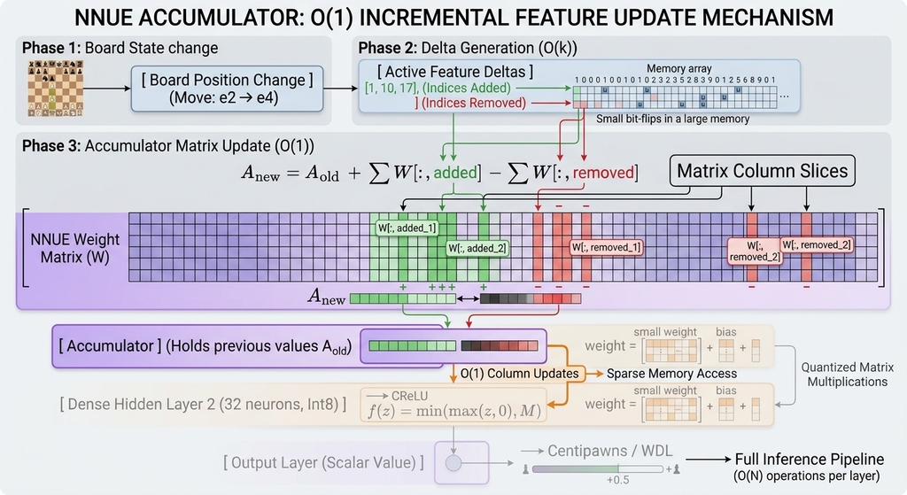
During game-tree search algorithms like Alpha-Beta pruning, millions of board states are evaluated per second. If a network required a full forward pass from scratch—evaluating all active features against the input matrix W_1—the computational cost would be proportional to the number of active pieces multiplied by the hidden dimension: O(|x|_0 \cdot h) or even O(d \cdot h) for dense layers.
NNUE bypasses this computational bottleneck by maintaining an accumulator state A in memory for each node in the search tree. Because consecutive board states in a search tree differ by only a local move (typically changing 2 to 4 board features—such as a piece leaving its old square and arriving on a new square, plus potential captures), the accumulator is updated differentially in O(1) time.
Mathematical Formulation of State Transitions
Let the sparse binary feature vector at search depth node t be denoted as x^{(t)}, and its corresponding accumulator vector be A^{(t)}.
When a move is executed, transitioning the board from state t to state t+1, the sparse input vector changes by activating a set of new feature indices \mathcal{I}<em>{\text{added}}</em> and deactivating a set of old feature indices <em>\mathcal{I}</em>{\text{removed}}:
x^{(t+1)} = x^{(t)} + \sum_{j \in \mathcal{I}_{\text{added}}} e_j - \sum_{k \in \mathcal{I}_{\text{removed}}} e_kWhere e_j represents the standard basis vector for feature index j.
Substituting this into the first-layer affine transformation:
A^{(t+1)} = W_1x^{(t+1)}+b_1=W_1 \left( x^{(t)} + \sum_{j \in \mathcal{I}_{\text{added}}} e_j - \sum_{k \in \mathcal{I}_{\text{removed}}} e_k \right) + b_1By distributing the matrix multiplication and recognizing that W_1 e_j corresponds exactly to the j-th column of matrix W_1 (denoted as W_{1, :, j}), the update equation simplifies to:
A^{(t+1)} = \left( W_1 x^{(t)} + b_1 \right) + \sum_{j \in \mathcal{I}_{\text{added}}} W_{1, :, j} - \sum_{k \in \mathcal{I}_{\text{removed}}} W_{1, :, k}Thus, the new accumulator is computed entirely via vector addition and subtraction:
A^{(t+1)} = A^{(t)} + \sum_{j \in \mathcal{I}_{\text{added}}} W_{1, :, j} - \sum_{k \in \mathcal{I}_{\text{removed}}} W_{1, :, k}This operation complexity depends exclusively on the number of changed features \mathcal{I}<em>{\text{added}}| + |\mathcal{I}</em>{\text{removed}}| (typically \Delta \le 4), completely independent of total feature dimensionality d.
Handling Complex Moves: Captures, Promotions, and Castling
While quiet moves simply remove the piece from its origin square and add it to the destination square (affecting features relative to both players’ kings), complex chess rules introduce multi-feature state transitions:
- Captures: When a piece is captured, it is removed from the board. This requires deactivating both the moving piece’s old feature relation and the captured piece’s feature relation on the target square.
- Pawn Promotions: A pawn transforming into a queen deactivates the pawn feature and activates the corresponding queen feature at the same coordinate.
- Castling: Castling involves two pieces moving simultaneously (the King and the Rook). The update delta must sum the added columns and subtract the removed columns for both pieces across their respective origin and destination squares.
Memory Layout and Cache Efficiency
Maintaining accumulators across a deep alpha-beta search tree requires a dedicated stack structure (the search stack). When the engine descends into a child node, it copies or updates the accumulator in place; when it backtracks (undoes a move), the accumulator state is restored instantly without recalculation.
To prevent memory bandwidth bottlenecks, weight matrices W_1 and accumulator buffers are aligned in CPU cache lines (typically 64 bytes), ensuring that vector additions execute with minimal cache misses.
Hardware Optimization and SIMD Vectorization (AVX2)
The Bottleneck: Scalar Arithmetic vs. Memory Bandwidth
The defining constraint of NNUE is achieving millions of evaluations per second on a commodity CPU using only alpha-beta search threads, without relying on external GPUs. While the incremental update (Section 4) handles the first layer efficiently, the subsequent dense layers (Layers 3, 4, and 5) require full matrix-vector multiplications for every evaluation.
Executing these dense layers using standard scalar assembly instructions (e.g., loading one 32-bit float, multiplying it, adding it to a register, repeating) would destroy search throughput. The CPU would spend most of its time waiting for data to arrive from RAM or the L3 cache, and the ALU (Arithmetic Logic Unit) would be severely underutilized.
NNUE solves this by heavily utilizing Advanced Vector Extensions 2 (AVX2), a Single Instruction, Multiple Data (SIMD) instruction set found in modern x86 CPUs.
Why Integers? Quantized Integer Arithmetic
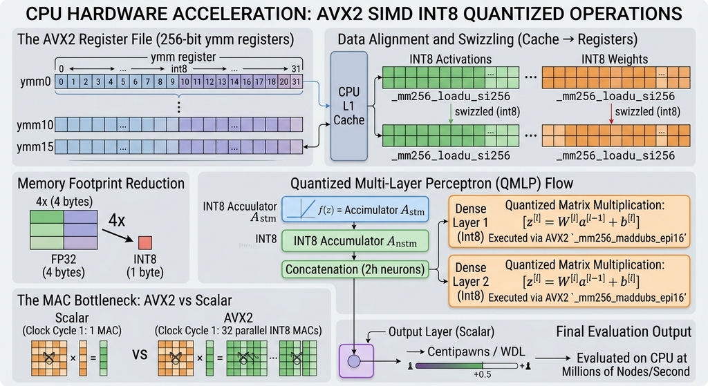
To leverage AVX2 effectively, NNUE does not use floating-point numbers (FP32) for its weights or activations in the dense layers. Instead, it operates entirely on quantized integers (typically int8 and int16).
Reasons for Using Integers:
- 4x Memory Footprint Reduction: An
FP32number consumes 4 bytes; anint8consumes 1 byte. Quantizing to 8-bit integers allows 4x more parameters to fit within the CPU’s critical L1 and L2 caches, maximizing cache locality and reducing expensive RAM access latency. - Parallelism via Packing: Since an AVX2 register is 256 bits wide, it can be “packed” with multiple integer values. A single 256-bit register can hold:
- 8
FP32floats (32 bits each). - 16
int16integers (16 bits each). - 32
int8integers (8 bits each).
- 8
- Throughput of Integer MAC Operations: Modern CPUs can execute integer Multiply-Accumulate (MAC) instructions with significantly higher throughput and lower latency than their floating-point equivalents. A single AVX2 instruction can multiply 32 pairs of
int8numbers and accumulate the results in one clock cycle.
Technical Implementation of AVX2 Intrinisics
NNUE engines utilize C/C++ SIMD Intrinsics to interact directly with the 256-bit ymm0–ymm15 registers. To achieve elite-level search speeds in game engines without sacrificing the non-linear representational power of neural networks, NNUE relies heavily on SIMD (Single Instruction, Multiple Data) parallelization. During the forward pass of quantized multi-layer perceptron (QMLP) layers, the engine must compute inner products between signed 8-bit integer weight matrices and quantized activations.
Writing this in standard scalar C would saturate the Arithmetic Logic Unit (ALU) and stall execution due to memory latency. By leveraging Intel’s AVX2 (Advanced Vector Extensions 2) instruction set, the CPU can load 256 bits of data into a single ymm register and perform parallelized integer multiply-accumulate (MAC) operations across multiple data lanes simultaneously. The C/C++ implementation below demonstrates how low-level hardware intrinsics are utilized to accelerate the core matrix-vector multiplication loops of an NNUE layer.
C code:
#include <immintrin.h>
#include <stdint.h>

// Compute dot product of quantized INT8 weights and INT8 activations using AVX2 in C
int32_t avx2_quantized_dense_layer_c(const int8_t* weights, const int8_t* inputs, int size) {
    __m256i acc = _mm256_setzero_si256();
    int i = 0;

    // Process 32 bytes per iteration using 256-bit AVX2 registers
    for (; i <= size - 32; i += 32) {
        // Load 32 bytes (256 bits) of weights and inputs unaligned from memory
        __m256i w = _mm256_loadu_si256((const __m256i*)(weights + i));
        __m256i in = _mm256_loadu_si256((const __m256i*)(inputs + i));

        // _mm256_maddubs_epi16 multiplies signed 8-bit ints by unsigned 8-bit ints,
        // producing 16-bit intermediate sums. We mask inputs to treat them as unsigned.
        __m256i product = _mm256_maddubs_epi16(_mm256_and_si256(in, _mm256_set1_epi32(0xFF)), w);

        // Accumulate 16-bit products into 32-bit integers using _mm256_madd_epi16
        acc = _mm256_add_epi32(acc, _mm256_madd_epi16(product, _mm256_set1_epi16(1)));
    }

    // Horizontal reduction: sum the 8 lanes of the 32-bit accumulator register
    int32_t buffer[8];
    _mm256_storeu_si256((__m256i*)buffer, acc);
    int32_t total = 0;
    for (int j = 0; j < 8; ++j) {
        total += buffer[j];
    }

    // Tail cleanup: process remaining elements that do not fit into a 32-byte chunk
    for (; i < size; ++i) {
        total += (int32_t)weights[i] * (int32_t)inputs[i];
    }

    return total;
}
C++ code:
#include <immintrin.h>
#include <cstdint>

// Compute dot product of quantized INT8 weights and INT8 activations using AVX2
int32_t avx2_quantized_dense_layer(const int8_t* weights, const int8_t* inputs, int size) {
    __m256i acc = _mm256_setzero_si256();
    int i = 0;

    // Process 32 bytes per iteration using 256-bit AVX2 registers
    for (; i <= size - 32; i += 32) {
        // Load 32 bytes (256 bits) of weights and inputs unaligned from memory
        __m256i w = _mm256_loadu_si256(reinterpret_cast<const __m256i*>(weights + i));
        __m256i in = _mm256_loadu_si256(reinterpret_cast<const __m256i*>(inputs + i));

        // _mm256_maddubs_epi16 multiplies signed 8-bit ints by unsigned 8-bit ints,
        // producing 16-bit intermediate sums. We mask inputs to treat them as unsigned
        // (common for ReLU/SCReLU activations).
        __m256i product = _mm256_maddubs_epi16(_mm256_and_si256(in, _mm256_set1_epi32(0xFF)), w);

        // Accumulate 16-bit products into 32-bit integers using _mm256_madd_epi16
        // to prevent arithmetic overflow across multiple iterations.
        acc = _mm256_add_epi32(acc, _mm256_madd_epi16(product, _mm256_set1_epi16(1)));
    }

    // Horizontal reduction: sum the 8 lanes of the 32-bit accumulator register
    int32_t buffer[8];
    _mm256_storeu_si256(reinterpret_cast<__m256i*>(buffer), acc);
    int32_t total = 0;
    for (int j = 0; j < 8; ++j) {
        total += buffer[j];
    }

    // Tail cleanup: process remaining elements that do not fit into a 32-byte chunk
    for (; i < size; ++i) {
        total += static_cast<int32_t>(weights[i]) * static_cast<int32_t>(inputs[i]);
    }

    return total;
}
Technical implementation notes:
- 256-Bit Vector Registration (
__m256i):- The code utilizes 256-bit wide AVX2 vector registers (
__m256i), allowing the CPU to process 32 bytes of data concurrently per iteration. _mm256_loadu_si256is used to load unaligned arrays from memory into the vector registers safely, preventing segmentation faults if weight and activation pointers are not strictly 32-byte memory aligned.
- The code utilizes 256-bit wide AVX2 vector registers (
- Signed/Unsigned MAC Optimization (
_mm256_maddubs_epi16):- A critical bottleneck in neural network quantization is matching signed and unsigned types. The intrinsic
_mm256_maddubs_epi16takes signedint8weights and unsignedint8activations (derived from clipped ReLU functions), multiplies adjacent pairs, and widens them into intermediate signedint16values in a single instruction cycle. - A bitwise AND mask (
_mm256_and_si256(in, _mm256_set1_epi32(0xFF))) ensures that the activation bytes are treated strictly as unsigned values.
- A critical bottleneck in neural network quantization is matching signed and unsigned types. The intrinsic
- Overflow Prevention and Accumulation (
_mm256_madd_epi16):- Accumulating products directly in 16-bit registers would cause frequent arithmetic overflows during long dot-product sequences.
- The function passes the 16-bit intermediate products into
_mm256_madd_epi16, multiplying them by1and widening them further into a vector of signed 32-bit integers (acc), ensuring high numerical precision and safety.
- Horizontal Reduction and Tail Cleanup:
- After the main SIMD loop processes chunks of 32 bytes, the 8 lanes of the 32-bit
accregister are stored into a temporary stack buffer via_mm256_storeu_si256and summed horizontally to yield the final inner product subtotal. - A tail cleanup loop handles any remaining elements whose count is less than the 32-byte block size, maintaining full functional correctness regardless of layer dimension sizing.
- After the main SIMD loop processes chunks of 32 bytes, the 8 lanes of the 32-bit
Training Methodologies, Loss Formulations, and Engine Ecosystems
Training an Efficiently Updatable Neural Network (NNUE) requires aligning the network’s internal evaluation surface with the tactical realities of alpha-beta search trees or the strategic long-term outcomes of full games. In modern computer chess and game engine development, three primary training paradigms have emerged, each adopted by distinct engine families and open-source ecosystems.
Paradigm 1: Pure Search Distillation (Supervised Heuristic Imitation)
Core Mechanism
In Search Distillation, the neural network is trained entirely as a supervised regressor to mimic an existing evaluation mechanism (such as a deeper alpha-beta search or an established hand-crafted evaluation function). The engine does not need to play full games or track terminal results. Instead, large datasets of static board positions x_i (extracted from opening books, human master games, or random self-play traversals) are evaluated using a search algorithm to extract a precise heuristic score v_{\text{search}, i}.
Loss Function
The optimization objective is modeled via Mean Squared Error (MSE) regression against the search evaluation:
\mathcal{L}_{\text{distillation}}(\theta) = \frac{1}{N} \sum_{i=1}^{N} \left( f(x_i; \theta) - v_{\text{search}, i} \right)^2Key Engines and Projects Using This Approach
- Experimental and Custom NNUE Projects: Many independent developers and open-source datasets (such as large-scale public repositories like the Gigafish dataset containing billions of annotated positions) rely exclusively on search distillation to bootstrap networks quickly without implementing complex self-play game loops.
- Value-Function Distillation Pipelines: Used extensively when researching alternative architectures (such as CNN-Transformer hybrids mimicking Stockfish evaluations) where generating reinforcement learning self-play trajectories is computationally prohibitive.
Paradigm 2: Game Outcome Regression (Reinforcement Learning / Self-Play)
Core Mechanism
In this paradigm, the network learns directly from objective ground-truth feedback: the terminal outcome of complete self-play games. The engine plays matches against itself from start to finish. Every board position x_i encountered along a specific game trajectory inherits the ultimate match result: z_i \in {-1, 0, 1} representing loss, draw, or win.
Loss Function
The optimization function targets the discrete game outcome:
\mathcal{L}_{\text{outcome}}(\theta) = \frac{1}{N} \sum_{i=1}^{N} \left( f(x_i; \theta) - z_i \right)^2Key Engines and Projects Using This Approach
- Leela Chess Zero (Lc0): Heavily inspired by AlphaZero, Lc0 relies purely on reinforcement learning self-play combined with Monte Carlo Tree Search (MCTS). Its networks are trained to predict policy probabilities and terminal game outcomes (z), optimizing entirely through self-play generation without imitating classical alpha-beta evaluation metrics.
- Early Neural Chess Experiments: Pure reinforcement learning from scratch without teacher supervision.
Paradigm 3: The Hybrid Blended Loss (The Modern State-of-the-Art)
Core Mechanism
Modern high-performance engines realized that both methods possess distinct flaws when used in isolation: pure search distillation makes the network inherit the teacher engine’s blind spots and horizon effects, whereas pure outcome regression suffers from extreme target sparsity and high noise (e.g., a blunder on move 40 labels all 39 previous winning positions as a loss).
To resolve this, modern pipelines combine both targets into a blended loss function. For every training position, the engine records both the immediate search evaluation v_{\text{search}} and the final game outcome z.
Loss Function
The unified training objective is expressed as a weighted sum balancing tactical heuristic guidance against long-term strategic reality:
\mathcal{L}_{\text{hybrid}}(\theta) = \frac{1}{N} \sum_{i=1}^{N} \left[ w \cdot \left( f(x_i; \theta) - v_{\text{search}, i} \right)^2 + (1 - w) \cdot \left( f(x_i; \theta) - z_i \right)^2 \right]Where w \in [0, 1] represents the blending hyperparameter (typically heavily favoring search supervision, e.g., w \approx 0.6 \text{ to } 0.8).
Key Engines and Projects Using This Approach
Stockfish (Official NNUE Training Pipeline): Stockfish utilizes massive distributed self-play frameworks where games are played, positions are sampled, searched to generate dense evaluation targets ($v_{\text{search}}$), and paired with the final match outcome ($z$). This hybrid training schedule enables Stockfish NNUE files to achieve elite evaluation precision.
Quantization-Aware Training (QAT) Across All Paradigms
Regardless of whether an engine adopts distillation, outcome regression, or a hybrid loss, deploying the resulting network inside a high-speed CPU search requires Quantization-Aware Training (QAT). Because inference executes entirely via low-precision signed 8-bit integers (int8) to maximize AVX2 SIMD throughput, standard floating-point training (FP32) introduces catastrophic rounding errors during Post-Training Quantization (PTQ).
QAT simulates integer discretization directly during the backpropagation forward pass:
W_{\text{quantized}} = \text{round}\left( \frac{W}{\Delta} \right) \cdot \DeltaUsing the Straight-Through Estimator (STE), the non-differentiable rounding operator’s gradient is bypassed:
\frac{\partial \text{round}(w)}{\partial w} \approx 1This ensures network weights adapt specifically to the discrete integer grid they will inhabit during sub-microsecond CPU tree evaluations.
Large-Scale Public Datasets: The Lichess Evaluation Database
A critical enabler for developers implementing Search Distillation (Paradigm 1) without the computational overhead of running an independent self-play cluster is the availability of massive, pre-evaluated open-source datasets.
The premier example in computer chess is the Lichess Open Database Evaluation Files (lichess_db_eval).
Core Characteristics and Scale
- Massive Volume: The dataset contains hundreds of millions of unique chess positions (scaling past 400,000,000 entries).
- Stockfish Annotations: Every single position is paired with precise evaluation metrics generated by variants of Stockfish running across crowdsourced analysis pipelines.
- Data Schema: Stored in compressed formats (such as JSON lines compressed via
zstandard), each entry provides the Fen string alongside principal variations (PVs), node counts, search depths, and centipawn evaluation scores.
Practical Application for Custom NNUE Training
For developers building custom engines or experimenting with neural evaluation parameters:
- Direct Supervised Ingestion: Instead of writing custom multiprocessing code to generate self-play games and run local Alpha-Beta searches, developers can stream the Lichess evaluation database directly into an NNUE training pipeline.
- Immediate MSE Optimization: By parsing the Fen strings into sparse binary input features (x_i) and extracting the Stockfish evaluation score as the target (v_{\text{search}, i}), the network can immediately minimize the distillation loss:
\mathcal{L}_{\text{distillation}}(\theta) = \frac{1}{N} \sum_{i=1}^{N} \left( f(x_i; \theta) - v_{\text{search}, i} \right)^2- Overcoming Hardware Bottlenecks: This approach allows hobbyists and researchers to train competitive, highly generalized NNUE feature transformers and dense layers on commodity hardware using pre-computed master-level heuristic evaluations.
Numerical Challenges, Gradient Flow, and Training Instabilities
Training an NNUE model introduces unique numerical and architectural challenges. Because the architecture combines sparse binary inputs, custom activations like SCReLU (Squared Clipped ReLU), and aggressive quantization constraints (int8), minor instabilities in gradient propagation can lead to catastrophic network degradation, dead accumulators, or severe overfitting to search artifacts.
Sparse Gradient Flow and Dead Accumulators
The first layer weight matrix W_1 connects tens of thousands of sparse binary features (e.g., HalfKP features exceeding 40,000 dimensions) to the accumulator vector. And this can suppose a problem.
Because board states only activate a tiny fraction of features simultaneously (typically |\mathcal{I}| \le 32 active pieces and King relations), the columns of W_1 corresponding to rarely occurring or obscure piece-square combinations receive zero gradient updates across vast portions of training datasets. Conversely, heavily frequented squares receive massive, repetitive gradient updates.
This imbalance causes “dead features” or exploding columns in W_1, where inactive weights stagnate while active weights saturate, leading to severe numerical drift when quantized to int8.
Training frameworks employ adaptive learning rate scaling per feature based on feature frequency, alongside specialized weight initialization distributions that account for the sparse fan-in of the accumulator layer.
Gradient Clipping and Quantization Noise Amplification
When performing Quantization-Aware Training (QAT), gradients must pass through the non-differentiable rounding operator via the Straight-Through Estimator (STE):
\frac{\partial \text{round}(w)}{\partial w} \approx 1Discretizing weights into fixed integer bins introduces quantization noise. During backpropagation, large outlier gradients can push continuous weights across multiple integer quantization thresholds in a single update step, triggering erratic oscillations in the loss landscape.
Ti mitigate this problem, strict gradient norm clipping is enforced globally across all dense and sparse layers:
\Vert{}\nabla_{\theta} \mathcal{L}\Vert{}_2 \le C_{\text{max}}where C_{\text{max}} is empirically tuned (typically between 0.5 and 1.0) to prevent gradient spikes from destabilizing the low-precision integer grid.
Positional Overfitting and Memorization
Because training pipelines (such as those ingesting the Lichess evaluation database or large self-play suites) contain hundreds of millions of positions, an NNUE network has sufficient capacity to memorize tactical motifs rather than learning general positional principles.
Overfitting manifests when the engine evaluates random, noisy tactical positions with extreme confidence while failing to understand smooth, quiet positional evaluations.
Mitigation:
- Data Augmentation via Board Symmetries: Exploiting horizontal board flips (swapping files
athroughh) effectively doubles or quadruples dataset diversity without additional search costs. - Regularization and Weight Decay: Applying L_2 regularization to dense hidden layers prevents weight explosion in the small fully connected matrices.
- Noise Injection: Adding bounded Gaussian noise to search evaluation targets v_{\text{search}} prevents the network from overfitting to minor centipawn fluctuations caused by search horizon cutoffs.
Engine Integration and Search Tree Interfacing
Integrating an NNUE evaluation function into an engine’s Alpha-Beta or Principal Variation Search (PVS) tree introduces architectural constraints that go far beyond standard heuristic evaluation functions. Because NNUE inference operates at sub-microsecond latencies across millions of nodes per second, the interaction between the neural network, the search stack, and the Transposition Table (TT) must be optimized to prevent microarchitectural bottlenecks.
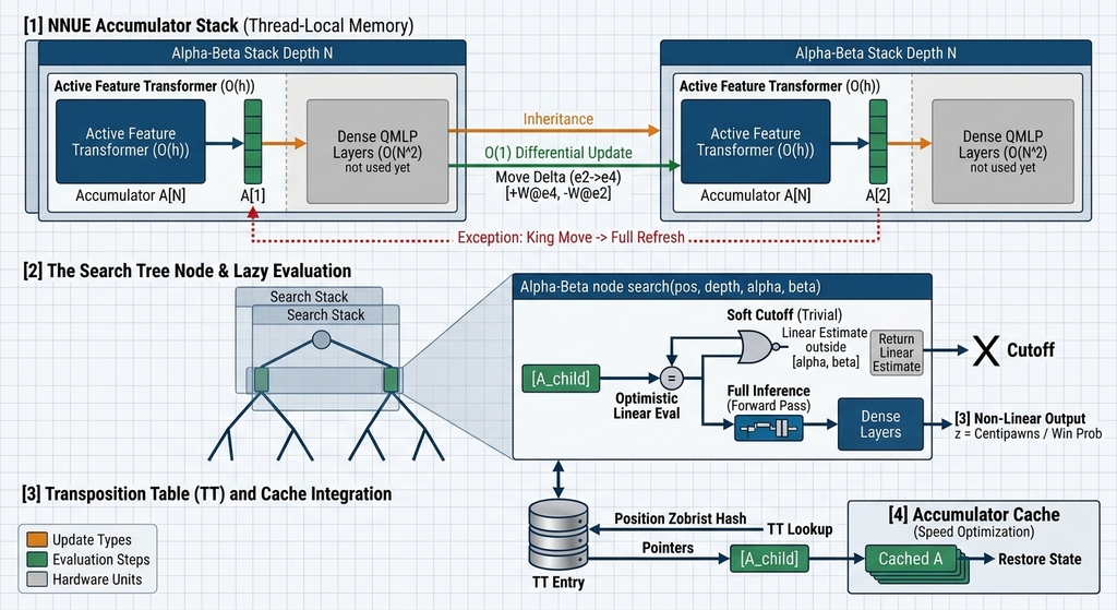
The Search Stack and Accumulator Lifecycle
To maintain the O(1) incremental update property, the engine maintains an Accumulator Stack aligned 1-to-1 with the search tree stack (SearchStack).
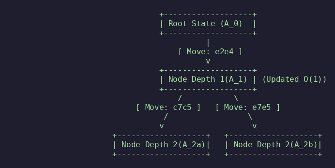
Memory Management Protocol
- Node Entry (Push): When the search tree branches into a child node via
search(pos, depth, alpha, beta), the engine creates a new search stack frame. The child node inherits the accumulator state A_{\text{parent}} of its parent. - Move Execution (Differential Update): The move’s feature additions (\mathcal{I}<em>{\text{added}}</em>) and subtractions (<em>[katex]\mathcal{I}</em>{\text{removed}}) are applied directly to compute A_{\text{child}} using AVX2 vector additions.
- King Movement Exception (Full Refresh): When a King moves, the relative coordinate system for the HalfKP/HalfKAv2 feature set shifts completely for that side. An incremental update becomes more expensive than recalculating the accumulator from scratch. In this scenario, the engine performs a Full Accumulator Refresh, re-evaluating all active piece positions for that color against W_1 in O(k \cdot h) time.
- Node Exit (Pop): When backtracking from a branch, the parent accumulator state remains untouched in its original stack frame, requiring zero cleanup operations.
Lazy Evaluation and Early Cutoffs
Even with AVX2 SIMD acceleration, computing the full forward pass of the dense layers (Layers 2 through 4) for every quiet node in the tree adds measurable overhead. Modern engines employ Lazy Evaluation to skip full neural inference when a node can be pruned based on trivial bounds.
Mathematical Formulation of NNUE Optimistic Bounds
Let \hat{v}_{\text{linear}} be an optimistic linear estimate computed directly from the accumulator magnitudes without passing through the non-linear quantized dense layers:
\hat{v}_{\text{linear}} = \sum_{j} w_j \cdot A_j + b_{\text{out}}If \hat{v}<em>{\text{linear}}</em> falls significantly outside the current search window [\alpha, \beta] by a conservative margin <em>M</em>{\text{lazy}}:
\hat{v}_{\text{linear}} + M_{\text{lazy}} \le \alpha \quad \text{or} \quad \hat{v}_{\text{linear}} - M_{\text{lazy}} \ge \betathe search can return \hat{v}_{\text{linear}} immediately or trigger a soft cutoff, bypassing the forward pass of the dense quantized layers entirely.
Interaction with Search Heuristics and Pruning Margins
Because an NNUE evaluation surface differs from classical hand-crafted evaluation functions (HCE)—exhibiting sharper non-linear tactical transitions—standard search pruning margins must be dynamically recalibrated.
Impact on Alpha-Beta Pruning Techniques:
- Futility Pruning: The condition v_{\text{eval}} + \text{margin}(\text{depth}) \le \alpha relies on stable evaluation bounds. NNUE evaluations can jump sharply across move boundaries due to sub-surface tactical awareness. Consequently, futility margins for NNUE are typically tighter than HCE margins.
- Null Move Pruning (NMP): If the NNUE evaluation is significantly above \beta (v_{\text{eval}} \ge \beta + R), the engine passes the turn (executes a null move). NNUE provides higher positional accuracy during null-move verification, reducing false positives in quiet positions.
- Late Move Reductions (LMR): LMR relies heavily on evaluation history and quiet move ordering. NNUE outputs are fused with move ordering heuristics (History Tables, Killer Moves, and SEE - Static Exchange Evaluation) to determine reduction depths.
Transposition Table (TT) Integration
The Transposition Table stores previously evaluated positions using 64-bit Zobrist keys. To prevent redundant NNUE forward passes across transposition hits:
- Evaluation Packing: NNUE evaluation scores are stored in TT entries using 16-bit packed integers, mapped directly from centipawn bounds or win-draw-loss (WDL) probabilities.
- Accumulator Cache Alignment: High-performance engines cache accumulator states inside TT memory structures or thread-local storage. When a position hash match occurs via a transposition, the engine can retrieve the pre-computed accumulator state directly, bypassing feature differential updates entirely.
Benchmarking, Performance Metrics, and Engine Elo Scaling
The primary objective of integrating NNUE is not simply to create a visually elegant evaluation function, but to drastically increase the playing strength (Elo rating) of the chess engine. Quantifying the precise impact of NNUE requires a rigorous benchmarking framework that separates computational efficiency (speed) from evaluation quality (understanding).
Measuring Inference Speed: Nodes Per Second (NPS)
The most direct metric for evaluating the efficiency of an NNUE implementation is its inference speed, measured in Nodes Per Second (NPS). NPS quantifies how many unique board positions the engine can evaluate every second during an actual game-tree search.
The Fundamental Trade-off
NNUE functions are significantly heavier computationally than classical hand-crafted evaluation (HCE) functions. When an engine switches from HCE to NNUE, its NPS typically drops by a significant factor (often 2x to 10x), because the CPU must execute vector instructions and matrix multiplications rather than simple table lookups.
\text{Performance Ratio} = \frac{\text{NPS}_{\text{HCE}}}{\text{NPS}_{\text{NNUE}}}The Evaluation Quality Paradox
A drop in NPS is only acceptable if the neural network’s evaluation is substantially more accurate than the classical heuristic. A stronger evaluation function allows the engine to make better decisions at a lower search depth. The key insight of NNUE success is: A small, deep search with excellent evaluation beats a massive, shallow search with mediocre evaluation.
Critical Latency Benchmarks for AVX2 Optimization
To achieve millions of NPS, the latency of a single NNUE forward pass across the dense quantized layers must be kept minimal. On modern CPUs, an optimized AVX2 execution of the dense layers (Layer 3, Layer 4, and Layer 5) should achieve sub-microsecond latency.
| Benchmark Operation | Target Latency (Microseconds) | Complexity | Hardware Resource |
| Incremental Update (quiet move) | \approx 0.05 \text{ to } 0.1 \mu s | O(\Delta) | L1 Cache, AVX ALU |
| Accumulator Refresh (King Move) | \approx 0.5 \text{ to } 1.0 \mu s | O(k \cdot h) | L1/L2 Cache, AVX ALU |
| Quantized Dense Pass (L3-L5) | \approx 0.2 \text{ to } 0.5 \mu s | O(h \cdot N_2) | AVX INT8 Throughput |
Table: Estimated target latencies for critical NNUE inference stages in a highly optimized AVX2 implementation.
Correlating Depth with Strength: The Elo vs. NPS Relationship
The relationship between the computational effort (search depth/time) and playing strength (Elo) follows an approximate logarithmic scaling law. The strength added by search decreases with each additional ply of depth.
\text{Elo Gain} \approx K \cdot \log_2\left(\frac{\text{T}_{1}}{\text{T}_{2}}\right)where K is a scaling constant, and T_{1}/T_{2} represents a doubling of the engine's speed (NPS) at a fixed search depth.
The NNUE Advantage in the Logarithmic Domain
Classical HCE engines might achieve 100 million NPS but face diminishing returns quickly because their evaluation can't solve complex positional tactical nuances. A 10 million NPS NNUE engine, despite having 1/10th the speed, has a higher ceiling: its evaluation surface is more non-linear and accurate. This allows it to find critical winning lines that HCE may only discover several plies later, more than compensating for the speed loss.
The Impact of Stockfish 12: A Case Study in NNUE Scaling
The release of Stockfish 12 marks the defining moment of the NNUE era. Stockfish, which already possessed the strongest HCE evaluation function in history, integrated an optimized NNUE inference engine into its existing Alpha-Beta framework.
The results, shown in Figure 9.1, were dramatic: a performance jump exceeding +100 Elo points, a massive gain at the elite level of engine development. This single update proved that neural network integration—when carefully optimized for sub-microsecond CPU inference—is the dominant strategy for modern game-playing AI.
\text{Elo}_{\text{Stockfish 12 (NNUE)}} \approx \text{Elo}_{\text{Stockfish 11 (HCE)}} + 100This scaling success triggered an "NNUE Revolution," leading almost every competitive chess engine (e.g., Komodo Dragon, Ethereal, Caissa) to adopt highly optimized quantized integer networks.
Alternative Architectures, HalfKA, and Theoretical Limits
While the standard HalfKP-based, quantized architecture remains the dominant solution for high-performance CPU inference (as seen in Stockfish), the NNUE field is rich with alternative topological designs and theoretical questions. These alternatives seek different balances between representation power (how well the network understands complex positions) and execution speed (the complexity of the AVX2 forward pass).
Feature Set Evolution: From HalfKP to HalfKA and Beyond
The feature set \mathcal{I} defines the "vocabulary" through which the neural network perceives the board.
HalfKP (The Standard): King and Piece Pairs
HalfKP (Half King-Piece) encodes the relationship between each side’s king and all other pieces. For example,
is a single feature. This set is sparse, updating only O(1) moves, and highly effective for king safety and pawn structure.
HalfKA (The Advanced): King and All Piece Pairs
HalfKA (Half King-All Pieces) expands this concept. It includes relationships between the King and pairs of other pieces, such as (\text{White King on g1}, \text{White Rook on f3}, \text{Black Queen on a5}).
An important concept is the complexity Trade-off: the HalfKA feature space is vastly larger (millions of dimensions rather than tens of thousands). While theoretically much more descriptive of complex tactics, the memory footprint of the sparse weight matrix W_1 becomes enormous, leading to cache misses and a severe NPS penalty that usually outweighs the accuracy gain.
Architectural Variations in Quantized Dense Layers
Beyond changing the input sparse features, developers experiment with the internal composition of the non-linear "dense" section of the network (Layer 3 to Layer 5).
Deepening the Network (L5, L6, L7+)
The classical NNUE is shallow (5 layers total). Deepening the network by adding more quantized hidden layers allows it to learn more complex hierarchical concepts (e.g., intermediate endgame principles).
The BottleNeck: Each additional layer adds non-linear quantized stages (SCReLU, QuantRound) that must be executed using AVX2. This increases the micro-second latency per inference. Deepening the network from L5 to L7 might improve evaluation accuracy but often drops NPS so severely that the engine’s overall playing strength decreases. The shallow network optimized for maximum AVX throughput is the "Goldilocks zone."
Varying the Accumulator Size (h)
The width of the accumulator (number of columns in W_1 and inputs to Layer 3), denoted by h, is a critical hyperparameter. Standard configurations use h=512 or h=1024.
The effect: increasing h improves the network’s capacity, but directly increases the number of AVX2 instructions required for both the differential update and the Layer 3 MADD operations. Halving h from 1024 to 512 roughly doubles the NPS but significantly decreases the evaluation precision in complex positions.
Theoretical Limits and the Horizon Effect
The fundamental limit of NNUE is architectural, not statistical.
The Curse of Quantization Noise
NNUE’s speed relies on integer arithmetic. To prevent numerical overflow and maximize speed, the network must use strict int8 quantization for all dense weights and inputs. This constraint acts as a severe information bottleneck. Even with Quantization-Aware Training (QAT), the network’s representation power is bounded by the discrete nature of the integer grid. Complex floating-point concepts cannot be perfectly mapped into int8, capping the network’s theoretical maximum accuracy compared to larger, higher-precision deep models (like Lc0’s FP32 CNNs).
NNUE vs. Lc0: The Scaling War
The computer chess landscape is a war between two philosophies: Depth vs. Evaluation.
\text{Playing Strength} = \text{Evaluation Accuracy} \cdot \log_2(\text{Search Depth})Lc0 (Monte Carlo Tree Search + CNN): Focuses on near-perfect evaluation accuracy. Its networks are massive, deep, and run on GPUs. Lc0 achieves extremely high evaluation accuracy at very low search depth (|\text{Depth}| \le 20).
Stockfish (Alpha-Beta Search + NNUE): Focuses on massive search depth. Its network is shallow, fast, and runs on CPUs. It achieves decent evaluation accuracy at massive search depth (|\text{Depth}| \ge 35).
The theoretical limit of NNUE is determined by how well a fast, shallow network can keep pace with an incredibly deep search, versus how well a massive, accurate network can survive a very shallow search. The success of Stockfish 12 proved that for Alpha-Beta, the "Depth + Quantized Neural Eval" strategy is currently the dominant paradigm for maximizing competitive Elo.
Hardware Deployment, CPU SIMD Optimization, and Future Directions
Deploying an NNUE model into a production chess engine requires maximizing execution throughput across diverse hardware platforms. Because NNUE relies on high-speed CPU inference rather than dedicated GPU compute, optimizing SIMD instruction sets, managing memory layouts, and adapting to modern SIMD ISAs (such as AVX-512, ARM NEON, and WebAssembly) dictates real-world search speed.
Microarchitectural Optimization across CPU Instruction Sets
The performance of NNUE scales directly with the width and vector capability of the target processor's execution units.
x86 Vector Extensions: AVX2 vs. AVX-512 / VNNI
While AVX2 remains the universal baseline for high-performance desktop engine builds, modern server and client CPUs support wider instruction sets:
- AVX-512 Vector Extensions: Increases vector width from 256 bits to 512 bits (
zmmregisters). Doubling register capacity allows processing 64 signed/unsigned 8-bit integers per instruction. - Vector Neural Network Instructions (VNNI): Introduces fused dot-product instructions like
vpdpbusd. In standard AVX2, multiplying unsigned bytes by signed bytes and accumulating into 32-bit integers requires two separate instructions (_mm256_maddubs_epi16followed by_mm256_madd_epi16). VNNI fuses this entire multiply-accumulate operation into a single clock cycle instruction, nearly doubling dense layer execution throughput.
Mobile and Edge Accelerators: ARM NEON
On mobile devices (iOS, Android, Apple Silicon ARM chips), NNUE executes via ARM NEON 128-bit vector registers:
- Multiply-accumulate operations rely on instructions such as
vdot_s32(Dot Product extension), which computes four 8-bit dot-products and accumulates into a 32-bit vector element in one step. - Proper memory alignment and cache prefetching (
__builtin_prefetch) are crucial to avoid bus stalls when updating accumulators across ARM's unified memory architectures.
SIMD Throughput Comparison across Architectures
| Instruction Set Architecture | Register Width | Operations Per Cycle (int8 MACs) | Key Hardware Intrinsics | Target Execution Speed |
| SSE4.1 / SSSE3 | 128-bit | 16 | _mm_maddubs_epi16 | Baseline / Legacy PCs |
| AVX2 | 256-bit | 32 | _mm256_maddubs_epi16 | Standard Commodity CPU |
| AVX-512 + VNNI | 512-bit | 64 | _mm512_dpbusd_epi32 | High-End Workstation / Server |
| ARM NEON (DotProd) | 128-bit | 16 | vdotq_s32 | Mobile / Apple Silicon |
| WASM SIMD128 | 128-bit | 16 | wasm_i16x8_extadd_pairwise_i8x16_s | Web-Based Analysis Tools |
Table: Vectorization capabilities and intrinsics across modern CPU microarchitectures.
Memory Layout, Alignment, and Cache Optimizations
Even the fastest SIMD vector instructions will stall if memory access is non-sequential or misaligned. Modern NNUE implementations employ strict cache-aware data structures:
- 32-Byte / 64-Byte Data Alignment: All accumulator arrays and weight matrices are aligned on 32-byte (for AVX2) or 64-byte (for AVX-512) boundaries using platform-specific allocators (
_mm_mallocorposix_memalign). Aligned loads (_mm256_load_si256) execute faster and avoid cross-cache-line penalties compared to unaligned loads (_mm256_loadu_si256). - Weight Matrix Transposition: Linear layer weight matrices W are stored in column-major memory order (transposed relative to standard mathematical layout). This guarantees that the 32 contiguous weights multiplied against input activations reside in a single contiguous memory block, allowing optimal SIMD streaming into vector registers without scatter-gather operations.
- L1/L2 Cache Pinning: Because the dense quantized layers are evaluated millions of times per second, their weight parameters are kept compact (often less than a few megabytes) to remain permanently pinned inside the CPU’s ultra-fast L1 and L2 caches.
Future Directions: Heterogeneous Engines and Dynamic Networks
As chess engine hardware and algorithms continue to evolve, NNUE research is branching into several promising avenues:
- Multi-Net / Dynamic Subnetworks: Engines like recent Stockfish releases utilize dynamic evaluation topologies. Instead of using a single large network, the engine dynamically selects between a small, fast network (for quiet or easily decided positions) and a large, expressive network (for complex tactical middle-games), optimizing the NPS-to-accuracy balance on a per-node basis.
- Feature Refinement (Threat & Pawn Inputs): Input representation is advancing beyond basic piece-square positions. Modern architectures (such as SFNNv16) experiment with threat-aware features (explicitly encoding attacked/defended pieces) and pawn-pair interactions, granting the network immediate spatial awareness before passing values to dense layers.
- CPUs vs. Hybrid GPU Offloading: While pure MCTS engines (Lc0) rely entirely on GPUs, modern NNUE research explores hybrid models where micro-NNUEs run on the CPU during alpha-beta search, while asynchronously querying larger GPU-based transformer models for global strategic evaluation at key branch nodes.
Conclusion
The introduction of Efficiently Updatable Neural Networks (NNUE) represents one of the most remarkable architectural milestones in the history of computer chess and heuristic search engines. For decades, the field was divided between two seemingly incompatible philosophies: high-speed, deep alpha-beta search engines powered by rigid hand-crafted evaluations, and slow, deep-learning-driven Monte Carlo tree search networks requiring massive GPU clusters. NNUE shattered this dichotomy by proving that neural network evaluation and high-speed CPU search can coexist in absolute harmony.
By combining sparse binary feature transformers with incremental updates, hardware-level AVX2 and VNNI vectorization, and robust training methodologies like search distillation and hybrid loss functions, modern engines achieve the best of both worlds. They retain the staggering calculation depth of alpha-beta search while gaining the nuanced, non-linear tactical awareness of a neural network.
Ultimately, NNUE bridges the gap between brute-force calculation and genuine positional intuition. Whether you are building a custom chess engine from scratch, optimizing SIMD intrinsics for microsecond inference, or experimenting with massive public datasets, diving into the world of neural evaluation opens up a fascinating, deeply rewarding frontier in computer science and artificial intelligence. We hope this guide serves as a solid foundation and inspires you to explore, experiment, and push the boundaries of what automated game engines can achieve!
Bibliography
- Nasu, Y. (2018). NNUE: Efficiently Updatable Neural Network for Shogi Evaluation Functions.
- Study of the Proper NNUE Dataset & A Theoretical Analysis of NNUE Design Principles (2024–2025). arXiv:2412.17948.
- Jacob, B., Kligys, S., Chen, B., Zhu, M., Tang, M., Howard, A., Kalenichenko, D., & Adam, H. (2018). Quantization and Training of Neural Networks for Efficient Integer-Arithmetic-Only Inference. IEEE/CVF Conference on Computer Vision and Pattern Recognition (CVPR), pp. 2704-2713.
- Stockfish Development Team. Official Stockfish NNUE PyTorch Training Framework (
nnue-pytorch). GitHub repository: https://github.com/official-stockfish/nnue-pytorch - Stockfish Development Team. Official Stockfish Core Engine Codebase. GitHub repository: https://github.com/official-stockfish/Stockfish
- Lichess. Lichess Open Database Evaluation Files (
lichess_db_eval.jsonl.zst). https://database.lichess.org/ - Intel Corporation. Intel® 64 and IA-32 Architectures Software Developer’s Manual Volume 2: Instruction Set Reference.
- Fog, A. Optimizing Software in C++: An Analysis of Instruction Latencies, Throughput and Microarchitecture Execution Units. Technical University of Denmark.